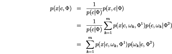
 , our objective is to maximize over
 Discrete context models are well established and successful tools with which to model or compress natural language text. These models predict the next letter, conditioned on the last few letters seen.
When the data are continuous, as in speech recognition or image processing, the situation is more complicated because one cannot rely upon exact context matches. As a result, context is typically either ignored, resulting in weak models, or it is incorporated in a way that is in some sense technically unsatisfactory, i.e. the contexts overlap so that the future is in effect used to predict the past.
This chapter discusses the learning of context models for continuous problem domains within a strict probabilistic framework. The probability of a time series, or of a static object such as an image, is expressed as a product of conditional probabilities. Each term predicts a never-before-seen part of the observation conditioned on earlier-seen portions. Models of this form are referred to in the literature as causal.
Our focus is on such models where each term arises by conditionalizing a mixture of primitive models, e.g. a conditionalized mixture of normal densities. We show that reestimation of such a model's parameters may be reduced to two simpler tasks. In the case of normal densities one of these is trivial, and the other may be approached the emphasis parameterization introduced in the previous chapter.
Now in the case of normal mixtures one might instead use a conventional gradient descent approach and a standard parameterization. Our contribution is the identification of a particularly simple, generic, and in some sense natural alternative.
In the case of a time series (e.g. a speech signal) the objective is usually to learn the parameters of a single conditional model that is then applied repeatedly to evaluate the probability of a series. For static objects such as images of handwritten digits, one might instead associate a different conditional model with each pixel position. The image's probability is then the product of the predictions made by these distinct models.
The original motivation for this work was in fact the learning of improved causal models for images - in particular of handwritten symbols. The developments of this chapter may form the basis for future experiments in this direction.
Given a collection of pairs ![]() where
where
![]() and
, our objective is to maximize over
and
, our objective is to maximize over ![]() :
:
We begin by observing that if the model is a single multivariate normal density, then this problem may be solved by instead optimizing the joint probability:
So the case of a single normal density is in a sense uninteresting.
We remark that linear predictive speech coding (LPC) may be
viewed as such a model where  .
.
In general these simple conditional forms arising from a single
normal density form a prediction ![]() based on a linear transformation
of the conditioning information
based on a linear transformation
of the conditioning information ![]() . As such their expressive
power is limited. In particular they cannot deal with modality.
For example, the population of
. As such their expressive
power is limited. In particular they cannot deal with modality.
For example, the population of ![]() values may separate into two
obvious clusters, each leading to very different predictions for
values may separate into two
obvious clusters, each leading to very different predictions for ![]() .
A simple linear predictor cannot cope with this situation and will
instead make a single blended prediction.
.
A simple linear predictor cannot cope with this situation and will
instead make a single blended prediction.
By moving from single densities to mixture densities, nonlinear predictions result and modality can be addressed.
A general mixture may be written
to describe the joint density ![]() . Provided that each
component
. Provided that each
component
![]() has an associated conditional
form
has an associated conditional
form
 we may then write:
Such conditionalized mixture forms can capture modality because
their mixing coefficients ![]() are not constant.
That is, they depend on the context
are not constant.
That is, they depend on the context ![]() and the mixture stochastically
selects a component based on the context.
and the mixture stochastically
selects a component based on the context.
If each component is a normal density with fixed parameters, the IMM technique for adaptive estimation and tracking results [BSL93,BBS88]. From this perspective, our interest is in recovering the model's parameters from observations.
For a single normal density we have seen that an optimal conditional model may be formed by first forming an optimal joint model, and then conditionalizing - and that the optimal joint model is specified by the sample mean and covariance.
Building an optimal joint model for a mixture of normal densities is a non-trivial and heavily studied problem. The most popular approach is Expectation Maximization (EM) which is discussed in earlier chapters and is an iterative technique for climbing to a locally optimal model.
But the situation is worse yet for conditionalized mixture forms because it turns out that conditionalizing an optimal joint mixture model, need not result in an optimal conditional model.
If the underlying joint density is exactly a normal mixture of ![]() components,
then the optimal conditional density is of course just the
conditionalized form the joint density (by direct calculation).
But given a finite sample, and especially one that is explained
poorly by a normal mixture of
components,
then the optimal conditional density is of course just the
conditionalized form the joint density (by direct calculation).
But given a finite sample, and especially one that is explained
poorly by a normal mixture of ![]() components, the optimal
conditional model will in general be different.
components, the optimal
conditional model will in general be different.
To see this we offer the following argument sketch: suppose
that ![]() and
and ![]() are independent with
are independent with ![]() explained perfectly
by a
explained perfectly
by a ![]() element mixture. Then
element mixture. Then ![]() Now consider
equation 22. The
Now consider
equation 22. The ![]() terms are
constant in an optimal model for
terms are
constant in an optimal model for ![]() but instead are
conditioned on
but instead are
conditioned on ![]() in the equation. By modeling the joint
density
in the equation. By modeling the joint
density ![]() it will seldom be the case that these terms
are constant whence the resulting model is suboptimal. That
is, in the case of independence, the context should be
ignored.
it will seldom be the case that these terms
are constant whence the resulting model is suboptimal. That
is, in the case of independence, the context should be
ignored.
The next section further reveals the role of these a
posteriori class functions in the overall optimization. An
example serves to illustrate that the ML estimate does not
necessarily optimize a posteriori class probabilities.
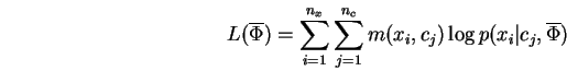
Consider figure 14(a) which depicts four points
along the x-axis, two ![]() labeled white and two
labeled white and two
![]() black. These colors correspond to two classes
black. These colors correspond to two classes ![]() and
and ![]() . The functions sketched above them represent
the ML normal density associated with each class. Notice the
mean of each is centered at the midpoint between each pair of
points, and that the variance is considerable. If one
computes, for example, the a posteriori probability
. The functions sketched above them represent
the ML normal density associated with each class. Notice the
mean of each is centered at the midpoint between each pair of
points, and that the variance is considerable. If one
computes, for example, the a posteriori probability
![]() based on the two normal densities shown, the
result will certainly exceed
based on the two normal densities shown, the
result will certainly exceed ![]() but clearly falls well
short of unity. If the densities are replaced with the more
peaked forms of the figure's part (b), all a posteriori
probabilities are in closer correspondence to the point colors.
This is true despite the fact that their means have drifted
away from the original midpoint locations. This illustrates
that ML optimization of a labeled dataset need not optimize
a posteriori class probabilities.
but clearly falls well
short of unity. If the densities are replaced with the more
peaked forms of the figure's part (b), all a posteriori
probabilities are in closer correspondence to the point colors.
This is true despite the fact that their means have drifted
away from the original midpoint locations. This illustrates
that ML optimization of a labeled dataset need not optimize
a posteriori class probabilities.
Figure 14 also illustrates the general concept of
emphasis introduced in the previous chapter since the
densities of part (b) may be generated by placing more weight
on points ![]() and
and 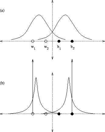 and computing the weighted mean and
variance. As the weight on these outer points is increased
the densities approach a pair of vertical pulses (also depicted)
and the a posteriori probabilities approach the ideal
values of zero or one in correspondence with each point's color.
and computing the weighted mean and
variance. As the weight on these outer points is increased
the densities approach a pair of vertical pulses (also depicted)
and the a posteriori probabilities approach the ideal
values of zero or one in correspondence with each point's color.
|
|
This section demonstrates how one may separate the parameter-learning task for conditional mixtures, into two simpler problems. This is accomplished using the mathematical machinery of EM combined with the introduction of new parameters.
Let ![]() denote the random variable being predicted/modeled,
and
denote the random variable being predicted/modeled,
and ![]() a random variable which conditions the prediction. To
simplify our notation we will generally use the single function
a random variable which conditions the prediction. To
simplify our notation we will generally use the single function
![]() to denote both probability densities and probabilities; as
well as related marginals and conditional forms. In all cases
it should be possible to distinguish different functions by
context. We begin by defining the central problem of this
chapter:
to denote both probability densities and probabilities; as
well as related marginals and conditional forms. In all cases
it should be possible to distinguish different functions by
context. We begin by defining the central problem of this
chapter:
 , or
announcing that a local minimum has been reached. That is,
maximize with respect to
, or
announcing that a local minimum has been reached. That is,
maximize with respect to
where the values ![]() and
and ![]() are members of some (possibly
finite) measure spaces.
are members of some (possibly
finite) measure spaces.
We remark that ![]() may be any non-negative function since
it may be normalized to form a probability function without
affecting the problem at hand. The MRCE problem as one step of
an iterative approach since it is not generally possible to
solve directly for even a local maximum of
may be any non-negative function since
it may be normalized to form a probability function without
affecting the problem at hand. The MRCE problem as one step of
an iterative approach since it is not generally possible to
solve directly for even a local maximum of
 .
.
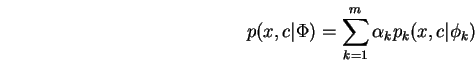
Our interest is in parameterized conditional densities
![]() which arise from finite mixture densities of the
form:
which arise from finite mixture densities of the
form:
where ![]() is a hidden discrete random variable which corresponds
to selection of a component of the mixture. We then write:
is a hidden discrete random variable which corresponds
to selection of a component of the mixture. We then write:
where it assumed that
![]() with
with
![]() . Were this not the case, we could make it
so by duplicating any common parameters. The resulting
parameterized density includes the original pdf as a special
case. So except for the matter of added model complexity,
our assumption that
. Were this not the case, we could make it
so by duplicating any common parameters. The resulting
parameterized density includes the original pdf as a special
case. So except for the matter of added model complexity,
our assumption that
![]() is made without harm6.1. The generation of a pair
is made without harm6.1. The generation of a pair
![]() may be thought of as a two stage process. First, a
pair
may be thought of as a two stage process. First, a
pair ![]() is chosen according to
is chosen according to ![]() Second,
Second, ![]() is generated according to
is generated according to ![]() and conditioned on the
earlier choice of
and conditioned on the
earlier choice of ![]() . Now
. Now
 from which we easily derive the conditional
prediction formula:
from which we easily derive the conditional
prediction formula:
Thus the conditional form required by the MRCE
problem arises naturally from the joint mixture density.
Next,
![]() , and as before we can without weakening
the model, assume that
, and as before we can without weakening
the model, assume that ![]() is made up of the
is made up of the ![]() marginal
values
marginal
values
![]() which we will sometimes denote
as just
which we will sometimes denote
as just ![]() , and
, and ![]() independently parameterized
densities
independently parameterized
densities
![]() . We will omit the
subscript on
. We will omit the
subscript on ![]() since it is clear from the conditioning on
since it is clear from the conditioning on
 what density we are referring to. We remark that
the same result may be reached by starting with the more
common definition of a mixture density:
what density we are referring to. We remark that
the same result may be reached by starting with the more
common definition of a mixture density:
where
![]() , the
, the ![]() are nonnegative, and
each
are nonnegative, and
each ![]() is a parameterized probability density function with
is a parameterized probability density function with
![]() . We prefer
our presentation however since it seems more natural given the structure
of later derivations.
. We prefer
our presentation however since it seems more natural given the structure
of later derivations.
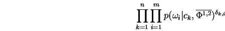
Now suppose that
![]() is an
independent sample of unlabeled observations where
is an
independent sample of unlabeled observations where ![]() denotes
denotes ![]() and
and ![]() denotes
denotes ![]() . Our approach
in this chapter is that of maximum-likelihood
estimation6.2, and we
are therefore interested in finding a value for
. Our approach
in this chapter is that of maximum-likelihood
estimation6.2, and we
are therefore interested in finding a value for ![]() which
maximizes
which
maximizes
![]() , i.e.
, i.e.
![]() . Such a value need not exist in general due
to degenerate cases such as zero variance distributions, but
we will not consider this complicating detail here. Since we
can equally well maximize the log-likelihood, we have the
following:
. Such a value need not exist in general due
to degenerate cases such as zero variance distributions, but
we will not consider this complicating detail here. Since we
can equally well maximize the log-likelihood, we have the
following:
The definitions above and much of the development that follows may be
generalized to the case where ![]() and or
and or ![]() are
measure spaces; in which case the summations become integrals. We
will however present the discrete case since it corresponds to our
original problem of parameter estimation given a finite sample.
are
measure spaces; in which case the summations become integrals. We
will however present the discrete case since it corresponds to our
original problem of parameter estimation given a finite sample.
We now show that the mixture-MRCE problem may be approached
by reducing it to an instance of itself with particular structure, and
multiple independent ordinary (nonmixture) MRCE problems. The ordinary
MRCE problems are simpler because each concerns only a single component
of the original mixture and excludes entirely the mixing coefficients
![]() . The mixture-MRCE subproblem is simpler because it
excludes the
. The mixture-MRCE subproblem is simpler because it
excludes the ![]() of the original problem, i.e. it concerns only the
model
of the original problem, i.e. it concerns only the
model
![]() .
.
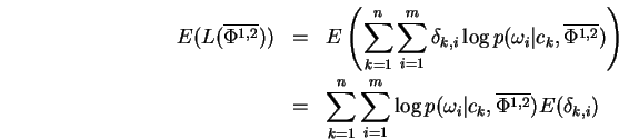
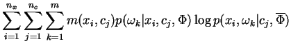
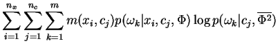
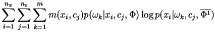
Proof: Using the same steps used derive the well-known EM algorithm, we have:
Reordering the summations in Eq-23 and grouping yields:
which after normalization of the bracketed term is easily recognized
as an instance of the mixture-MRCE problem. The second term
Eq-24 making up ![]() may be similarly transformed to yield:
may be similarly transformed to yield:
which is just ![]() independent instances of the simple MRCE problem.
Finally, observe that Eq-6.2 and Eq-6.2 are independent
of one another since the first is an optimization problem over
independent instances of the simple MRCE problem.
Finally, observe that Eq-6.2 and Eq-6.2 are independent
of one another since the first is an optimization problem over
![]() and
the second over
and
the second over
![]() - completing our proof.
- completing our proof. ![]()
Notice that if ![]() contains a single value, the
complexities introduced by the conditional form of the problem
vanish and one is left with the standard EM setting in which
the mixture-MRCE subproblem is trivially maximized. Also, the
conditional estimation problem becomes a plain estimation
problem.
contains a single value, the
complexities introduced by the conditional form of the problem
vanish and one is left with the standard EM setting in which
the mixture-MRCE subproblem is trivially maximized. Also, the
conditional estimation problem becomes a plain estimation
problem.
For normal densities the conditional estimation problems of Eq-24 are easily solved since the optimal conditional normal density is obtained by finding the optimal joint density and then conditionalizing.
The MRCE problem of Eq-23 is however much more difficult. It, or for that matter the entire problem, might be addressed by gradient descent where the covariance matrices have been reparameterized to ensure positive definiteness. The purpose of this chapter is to describe an alternative approach.
Using the emphasis reparameterization results of the previous chapter, we may (except for degenerate cases) express a posteriori class behavior by reweighting the available samples.
So in particular Eq-23 may be approached in this way.
That is, the ![]() may be reweighted until the term is maximized.
This amounts to a reparameterization of the problem in terms of these
weights rather than in terms of means, covariance matrices, and mixing
coefficients.
may be reweighted until the term is maximized.
This amounts to a reparameterization of the problem in terms of these
weights rather than in terms of means, covariance matrices, and mixing
coefficients.
The fact that for normal densities one may pass easily from such a weight set, to an ML traditional parameter set, is essential to the approach. That it is capable of expressing the solution is also a special characteristic of normal densities (see previous chapter).
But in practice one might wish to use this reparameterization (without proof of expressiveness) for other densities for which an ML estimate of a weighted sample set is readily available. Its virtue is that the particular density may then be viewed as a data type referred to by a single optimization algorithm.
A particularly simple numerical prescription for optimization is that of Powell (see [Act70,Bre73,PFTV88]). Speed of convergence is traded for simplicity in that no gradient computation is required. Emphasis reparameterization does however introduce one wrinkle. The number of parameters can easily exceed the degrees of freedom in the underlying problem. In the case of normal mixtures, the number of natural parameters (i.e. mean vector values and covariance matrix entries) may be far less than the number of training samples available. In this case we propose to modify Powell's method to use an initial set of random directions with size matching the number of native parameters.
The result is a simple and highly general approach to estimating the parameters of conditional mixtures. That the approach can express the globally optimal parameter set has only been established for normal mixtures, but we expect that approach may nevertheless work well in other settings.
The conditional entropy minimization problem can express the traditional
problem of supervised learning given boolean ![]() with
with
![]() . That is, each datapoint has an
attached label. The MRCE problem is then to minimize the bits
required to express the labels, given the data. Our
definition of MRCE places no restriction, other than
non-negativity, on the
. That is, each datapoint has an
attached label. The MRCE problem is then to minimize the bits
required to express the labels, given the data. Our
definition of MRCE places no restriction, other than
non-negativity, on the ![]() . In this section we motivate
the form of our definition by showing that these weights have
a natural stochastic interpretation.
. In this section we motivate
the form of our definition by showing that these weights have
a natural stochastic interpretation.
Imagine a random process where each trial consists of drawing a
label from
![]() for each of the points
for each of the points
![]() . The outcome of each trial is represented by
boolean random variables
. The outcome of each trial is represented by
boolean random variables ![]() defined to be
defined to be ![]() if
if
 is observed to have label
 ![]() , and
, and ![]() otherwise.
No independence assumptions are made. The trials might be
time dependent; and within a trial, the labels might be
dependent in some complex way. Each trial produces a labeled
dataset with likelihood:
otherwise.
No independence assumptions are made. The trials might be
time dependent; and within a trial, the labels might be
dependent in some complex way. Each trial produces a labeled
dataset with likelihood:
Denoting by
 the logarithm of this likelihood,
a straightforward consequence of the linearity of expectations is then that:
the logarithm of this likelihood,
a straightforward consequence of the linearity of expectations is then that:
where the expectation is over trials of the random
labeling process. The key feature of this expression is that
the expectation of each labeled dataset's log likelihood, is
independent of the exact nature of the labeling process;
depending only on the individual expectations
![]() . The significance of this independence, is
that we can optimize
. The significance of this independence, is
that we can optimize
![]() with respect to
with respect to
![]() , where the only knowledge we have regarding the
labeling process is the set of terms
, where the only knowledge we have regarding the
labeling process is the set of terms
![]() .
Now
.
Now
![]() since only a single label
is drawn for each point. So
since only a single label
is drawn for each point. So
![]() as well. These
as well. These ![]() terms are therefore the
probability of observing label
terms are therefore the
probability of observing label ![]() given point
and correspond to the term
given point
and correspond to the term
![]() in
Eq-23. Because of the argument above, we think of
the weights as stochastic labels attached to each point.
in
Eq-23. Because of the argument above, we think of
the weights as stochastic labels attached to each point.
In the setting above, each trial can be thought of as drawing
a sample of size ![]() consisting of exactly
consisting of exactly
![]() each time. This is just one example of a process which draws
sample of size
each time. This is just one example of a process which draws
sample of size ![]() , from the
, from the ![]() with equal probability
with equal probability
![]() . An argument essentially the same as that above can
then be made for a process in which each trial draws a single
data point from
. An argument essentially the same as that above can
then be made for a process in which each trial draws a single
data point from
![]() and then a single label for
that point. By repeated trials, the sample of size
and then a single label for
that point. By repeated trials, the sample of size ![]() is
built. The result is that given only the probability of
drawing each , and the
is
built. The result is that given only the probability of
drawing each , and the ![]() , we can optimize
our expected log likelihood for a series of
, we can optimize
our expected log likelihood for a series of ![]() samples,
independent of the exact nature of the process.
samples,
independent of the exact nature of the process.
Now an equivalent problem results if our matrix of weights
![]() is scaled by a constant so that the
sum of its entries is
is scaled by a constant so that the
sum of its entries is ![]() , so we will assume that this is the
case. It can then be thought of a joint probability density
on
, so we will assume that this is the
case. It can then be thought of a joint probability density
on ![]() so that entry may be expressed as a product
so that entry may be expressed as a product ![]() . More formally,
. More formally, ![]() may be expressed as a diagonal
matrix with trace
may be expressed as a diagonal
matrix with trace ![]() representing
representing ![]() , times a row
stochastic matrix representing
, times a row
stochastic matrix representing ![]() .
.
In summary, an instance of the MRCE problem may be thought of
as consisting of
![]() and the stochastic knowledge
in the two matrices above. The significance of its solution
is that it represents a minimum not just over parameter
values, but over all processes consistent with this knowledge.
If our objective were to maximize expected likelihood rather
than expected log likelihood, this would not be true. Thus
beyond the obvious mathematical convenience of working with
log likelihood, there is a deeper benefit to doing so.
Everything we've said is true in a far more general sense for
arbitrary density
and the stochastic knowledge
in the two matrices above. The significance of its solution
is that it represents a minimum not just over parameter
values, but over all processes consistent with this knowledge.
If our objective were to maximize expected likelihood rather
than expected log likelihood, this would not be true. Thus
beyond the obvious mathematical convenience of working with
log likelihood, there is a deeper benefit to doing so.
Everything we've said is true in a far more general sense for
arbitrary density ![]() and sets
and sets ![]() and
and 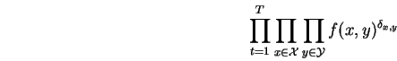 , where
we focus on a series of
, where
we focus on a series of ![]() samples and have the likelihood:
samples and have the likelihood:
but we will not repeat the argument above at this slightly more abstract level.
Instead we turn to a concrete example loosely motivated by the problem of portfolio optimization as framed in [Cov84] and discussed in chapter 2, in order to illustrate the mathematical point above.
Suppose that one may draw vectors from
![]() at random according to
some hidden distribution
at random according to
some hidden distribution ![]() , and that the one thing known about this
distribution is that only two values
, and that the one thing known about this
distribution is that only two values ![]() and
and ![]() are ever drawn in
each component position, and that they occur with equal probability in
each position. That is, all single variable marginals are known.
are ever drawn in
each component position, and that they occur with equal probability in
each position. That is, all single variable marginals are known.
Now focus on the product of a vector's components. Our expectation of
the ![]() of this product's value is zero because the product becomes
a sum of logs, and because of linearity of expectations.
of this product's value is zero because the product becomes
a sum of logs, and because of linearity of expectations.
Of significance is that the expectation is zero, independent of the nature
of ![]() . By contrast, our expectation of the product's value (without
taking the logarithm) is highly distribution dependent. For example,
if the distribution generates a vector of
. By contrast, our expectation of the product's value (without
taking the logarithm) is highly distribution dependent. For example,
if the distribution generates a vector of ![]() 's half of the time and
a vector of
's half of the time and
a vector of ![]() 's the rest of the time, the resulting expectation
is
's the rest of the time, the resulting expectation
is
![]() and is immense.
and is immense.
The fascinating observation regarding optimizing log-likelihood as opposed to likelihood, is that on the one hand the optimization is over a huge space of hidden distributions, but on the other hand the optimization ignores information in those distributions that can significantly affect the expected likelihood.
We conclude by identifying and briefly discussing a number of potential applications for conditional normal mixture models (CNM).
As mentioned earlier, our starting point was handwriting recognition and in particular the problem of offline digit classification. The space of digit images is modeled as a mixture of models, one for each digit. We suggest that each digit's model itself consist of a mixture of models intended to capture the sometimes very different styles used to represent the same numeral. Each digit style model would then consist of a product of CNMs, one for each pixel position, with conditioning on some subset of the earlier-seen pixels. The use of CNMs in this way promises to better model the variation that exists within a single style. The final model may be used to implement a traditional Bayesian classifier. The introduction of discriminative training into this framework is an interesting area for future work.
The same approach might be used in machine vision to build highly general statistical models for particular objects based on a set of training images. A classifier may then build as for handwritten digits. Applied to images CNMs might also find application in image restoration or perhaps in the area of digital water-marking.
Our development in chapter 2 showed that Baum-Welch/EM may be used to estimate the parameters of non-causal models as well. In many applications, including some of those mentioned above, a non-causal model may suffice. For images this corresponds to the modeling of a pixel using a context that entirely surrounds it. Baum-Welch/EM is certainly easier to implement than the approach of this chapter and may therefore represent the technique of choice when implementing non-causal CNM models.
Finally we point out that while this chapter has focused on ML estimation, techniques similar to those of chapter 2 might be developed to implement alternative estimation criteria.
![\begin{displaymath}
\sum_{k=1}^m \sum_{j=1}^{n_c}
\left [\sum_{i=1}^{n_x}
m(...
..._j,\Phi) \right]
\log p(\omega_k\vert c_j,\overline{\Phi^2})
\end{displaymath}](img836.gif)