Chapter 2 introduced the application of finite growth models to the problem of learning the parameters of stochastic transducers in rather general form, and considered the case of a string edit distance in greater detail. That is, a memoryless single state 2-way transducer.
In this chapter we establish the practical utility of this approach by learning an optimal string edit distance function from a corpus of examples and reporting on the performance of this function in a concrete application: the identification of words in conversational speech given a phonetic transcription and reference dictionary3.1. The function we learn exhibits one third the error rate of Levenshtein distance [Lev66]; the canonical untrained edit distance case. We first implemented the transduction at the heart of our approach in August 1993 for the problem of classifying grey-scale images of handwritten digits.
The speech recognition problem may be viewed as a transduction
![]() from a signal
from a signal ![]() to text
to text ![]() . The text is
typically regarded as a sequence of words from a fixed
vocabulary recorded in a lexicon
. The text is
typically regarded as a sequence of words from a fixed
vocabulary recorded in a lexicon ![]() . This transduction bridges
a wide representational gap and investigators commonly introduce
an intermediate phonetic language
. This transduction bridges
a wide representational gap and investigators commonly introduce
an intermediate phonetic language ![]() and the problem
is then viewed as
and the problem
is then viewed as
![]() .
.
Our experiments focus on the second segment
![]() .
Crossing the entire gap from
.
Crossing the entire gap from ![]() to
to ![]() through the learning
of multistage transductors represents an interesting area
for future work.
through the learning
of multistage transductors represents an interesting area
for future work.
We assume that ![]() is given and seek to identify the correct
corresponding sequence of words from
is given and seek to identify the correct
corresponding sequence of words from ![]() .
Moreover, we assume that the word boundaries within
.
Moreover, we assume that the word boundaries within ![]() are
known, and that
are
known, and that ![]() contains one or more valid phonetic spellings
for each word in the vocabulary.
contains one or more valid phonetic spellings
for each word in the vocabulary.
Our problem is then to accept a sequence of noisy phonetic
spellings taken from ![]() , and output the correct sequence of
words from
, and output the correct sequence of
words from ![]() . This problem has the virtue of being easily
stated but retains a strong connection to the original speech
recognition task.
. This problem has the virtue of being easily
stated but retains a strong connection to the original speech
recognition task.
The corpus we use is considered to be quite difficult and
indeed current systems exhibit an error rate of above 45% on
it. This is in contrast to error rates closer to 5% on
easier tests. We describe and evaluate several variations on a
basic model. The best of these exhibits an error rate of
slightly more than 15%, where we remind the reader that this
figure applies to the
![]() leg only and assumes
knowledge of word boundaries.
leg only and assumes
knowledge of word boundaries.
The phonetic spellings that form our input are generated by
human experts listening to ![]() . For this reason our results
might be viewed as an optimistic estimate of what is possible.
On the other hand, generation of the output word sequence
involves no high order language model; only the
probabilities of individual words are considered when forming
the output sequence. Such high order models are an important
factor in existing speech systems and might therefore
reasonably be expected to improve results under our approach.
Also, more sophisticated context sensitive transducers are
possible within our theoretical framework, and these also promise
to improve performance.
So despite our simplifying assumptions we submit that our
experimental results are of some practical significance to the
original problem.
. For this reason our results
might be viewed as an optimistic estimate of what is possible.
On the other hand, generation of the output word sequence
involves no high order language model; only the
probabilities of individual words are considered when forming
the output sequence. Such high order models are an important
factor in existing speech systems and might therefore
reasonably be expected to improve results under our approach.
Also, more sophisticated context sensitive transducers are
possible within our theoretical framework, and these also promise
to improve performance.
So despite our simplifying assumptions we submit that our
experimental results are of some practical significance to the
original problem.
Our generative model begins with the
choice of a word ![]() according to a simple probability
function on the vocabulary. Given
according to a simple probability
function on the vocabulary. Given ![]() a particular lexical
phonetic spelling
a particular lexical
phonetic spelling ![]() is selected from the alternatives
recorded in
is selected from the alternatives
recorded in ![]() - again according to a probability function.
Finally, a surface phonetic spelling
- again according to a probability function.
Finally, a surface phonetic spelling ![]() is generated
from
is generated
from ![]() via stochastic transduction - and in the case of our
experiments, using a single state memoryless transducer
corresponding to string edit distance. Note that the alphabet
used to express lexical phonetic spellings may differ from
that used to represent the surface phonetic spellings seen in
via stochastic transduction - and in the case of our
experiments, using a single state memoryless transducer
corresponding to string edit distance. Note that the alphabet
used to express lexical phonetic spellings may differ from
that used to represent the surface phonetic spellings seen in ![]() .
This model is written:
.
This model is written:
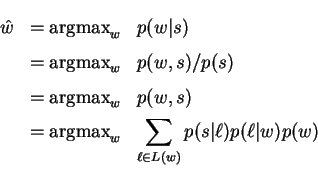
The issue is then one of estimating the parameters of this model
which were omitted from the notation above for simplicity. We now
begin using ![]() to denote them. They include the probability
function used to choose words, that used to choose lexical phonetic
spellings, and the transducer's parameters as well.
to denote them. They include the probability
function used to choose words, that used to choose lexical phonetic
spellings, and the transducer's parameters as well.
We are given a training set of pairs ![]() where
where ![]() is a vocabulary
word and
is a vocabulary
word and  its surface phonetic transcription.
Our learning objective is then to maximize over
 ![]() :
:
The test set consists only of surface phonetic forms, and we face the recognition problem described above which recovers a vocabulary word for each of these observed surface forms. This objective is recognized as an instance of the ML mixture density/function parameter estimation problem and we apply the expectation maximization (EM) [DLR77] as discussed in chapter 2.
Our implementation actually models the product
![]() as a single joint probability
as a single joint probability
![]() .
The initial parameters for this mixture and all edit distance
costs are uniform. A fixed value of
.
The initial parameters for this mixture and all edit distance
costs are uniform. A fixed value of ![]() is added to the
mixture's expectation accumulators as a statistical flattening precaution - preventing the probability of any
lexicon entry from being driven to zero during learning. No
effort was made to optimize this constant. Each EM iteration
replaces
is added to the
mixture's expectation accumulators as a statistical flattening precaution - preventing the probability of any
lexicon entry from being driven to zero during learning. No
effort was made to optimize this constant. Each EM iteration
replaces ![]() with new values.
with new values.
The a posteriori probabilities
![]() are
computed during EM for each
are
computed during EM for each ![]() and these are used
to weight the expectation steps taken for the conditional
transduction
and these are used
to weight the expectation steps taken for the conditional
transduction
![]() . Here we make the simplifying
assumption that this conditional form may effectively be maximized
by instead maximizing the joint transducer probability
. Here we make the simplifying
assumption that this conditional form may effectively be maximized
by instead maximizing the joint transducer probability
![]() so that we can directly apply the FGM-based
algorithm for learning string edit distance described in the
previous chapter. Strictly then the new
so that we can directly apply the FGM-based
algorithm for learning string edit distance described in the
previous chapter. Strictly then the new ![]() may not be an improvement
but empirically is.
may not be an improvement
but empirically is.
This approach to learning solves an important problem: that of
corresponding the observed surface phonetic form  with
the hidden lexical phonetic forms
 ![]() . Intuitively
. Intuitively
 is paired with the most likely
 ![]() and used to
train the transducer. Of course this matching is stochastic.
Later in this chapter we will see that the simpler approach of
merely training all possible pairs with equal emphasis results
in poor performance indeed.
and used to
train the transducer. Of course this matching is stochastic.
Later in this chapter we will see that the simpler approach of
merely training all possible pairs with equal emphasis results
in poor performance indeed.
The Switchboard corpus consists of over 3 million words of recorded telephone speech conversations [GHM95]. The variability resulting from its spontaneous nature makes it one of the most difficult corpora for speech recognition research. Current recognizers exhibit word error rates of above 45% on it - compared to rates closer to 5% on easier tests based on read speech. Switchboard also includes a lexicon with 71,200 entries using a modified Pronlex alphabet (long form) [LDC95].
Roughly 280,000 of Switchboard's over 3 million words have been phonetically transcribed manually by ICSI using a proprietary alphabet [GHE96].
Both the Switchboard lexicon and ICSI transcription were
filtered to make the two compatible.
We removed 148 entries from the lexicon that included unusual
punctuation ([<!.]). A total of 73,068 transcript
deletions were made as follows: 72,257 with no corresponding
valid syntactic word, 688 having empty phonetic transcript,
88 with an incomplete transcript, 27 and 8 that included
the undocumented symbols ? and ! respectively.
Note that symbols ? and ! are not part of
either alphabet (long forms) and are used only in the transcript.
The final lexicon used in our experiments contains 70,952 entries describing 66,284 syntactic words over an alphabet of 42 phonemes. The final transcript used in our experiments has 214,310 entries - 23,955 of which are distinct. These correspond to 9,015 syntactic words over 43 phonemes (32 Pronlex plus a special silence symbol). The transcript was divided 9:1 into 192,879 training and 21,431 test words.
We report on the results of 56 different experiments resulting from an exploration of several different degrees of freedom:
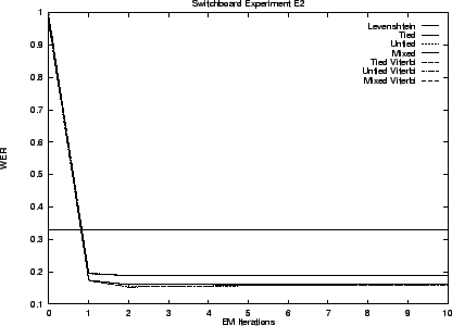
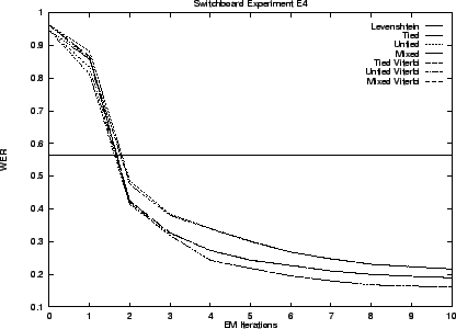
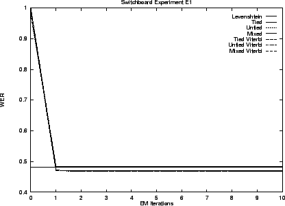
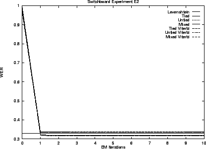
Our first set E1 of experiments uses the Switchboard lexicon. This lexicon contains many words that are never used in the ICSI transcript and experiment E2 replaces it with a lexicon containing only those 9,621 entries that correspond to words that do occur in the transcript.
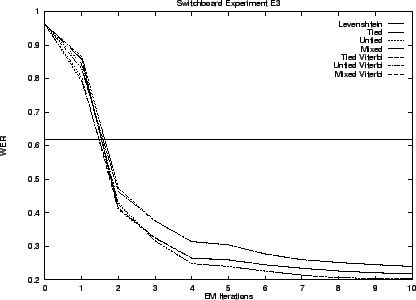
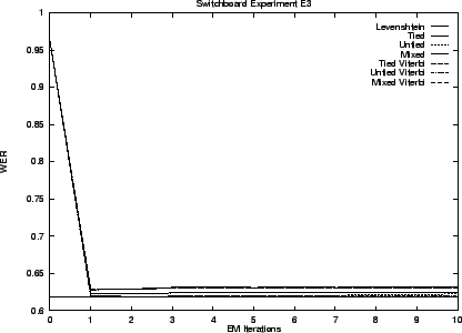
Experiments E3 and E4 leave the Switchboard lexicon behind and construct one instead from the ICSI transcript. Experiment E3 uses a lexicon built from the training transcript. It contains 22,140 entries for 8,570 syntactic words. The test transcript includes 512 entries that do not occur in this lexicon so that 2.4% represents an error rate floor for experiment E3. The lexicon for experiment E4 is built using the entire transcript and has 23,995 entries for 9,015 words.
We report the fraction of misclassified samples in the testing transcript, that is the word error rate. For each surface phonetic form in the test transcript, one or more syntactic words are postulated by the decision process. The fraction of correctly classified words is then the sum over the test transcript of the ratio of the number of correct words identified to the number of postulated words. The fraction misclassified is then one minus this fraction.
With nothing more said experiment E4 would seem to be uninteresting since its lexicon contains an exact match for each phonetic spelling present within the test transcript. One might therefore expect 100% accuracy from this experiment. But the lexicon contains a large number of homophones, that is different syntactic words that have at least one phonetic spelling in common. This arises from two sources. First, conventional phonetic alphabets have limited expressiveness, especially when applied to short words in rapidly articulated conversational speech. Second, in such speech, words frequently change their phonetic shape considerably and in so doing collide with other words. That these phenomena are significant is clearly demonstrated by our results (reported later) for experiment E4.
Three basic forms of string edit distance are compared in our
experiments. The simplest of these is the classic Levenshtein
prescription which assigns zero cost to identity substitutions
and unity cost to all other operations. Stochastic edit distance
is defined in chapter 2 as the negative logarithm
of the probability that two strings are simultaneously
grown using left-insertion, right-insertion, and joint-insertion
operations. This form effectively aggregates all transductions
between the two strings. Viterbi edit distance instead selects
only a single transduction (path through the FGM) of maximal
probability. It is then identical to conventional edit distance
where the edit costs are the negative logarithms of the corresponding
generative insertion probabilities. Note that by definition the
Viterbi edit distance can be no less than the stochastic edit distance.
Also observe that the Levenshtein form has no stochastic interpretation
strictly within our framework since infinitely many identity
substitutions is less costly than even a single unity cost operation.
The problem derives from the fact that its cost table includes
zero entries. Any such table is problematic. But given that
all entries are strictly positive, there is always an equivalent
stochastic Viterbi form. So in particular the Levenshtein form may
be approximated by assigning the zero cost operations some small
cost ![]() .
.
Levenshtein distance is parameter-free but may be viewed as having four parameters: identity substitution, nonidentity substitution, insertion, and deletion - set to 0, 1, 1, and 1 respectively.
Both the Viterbi and stochastic forms of edit distance are parameterized by their table of elementary operation costs. The number of such parameters is then usually much greater than four.
To determine if such fine control over costs is really necessary and justified by the available training data, we implement a tied form of both Viterbi and stochastic edit distance that reduces the parameter set to the four given above. Our Viterbi-tied form may then be viewed as a generalized Levenshtein-style prescription. This tying is easily implemented by simply summing over each category of operations during the maximization step.
Thus far we have defined five distance functions: Levenshtein, Viterbi distance (untied), Viterbi distance (tied), stochastic distance (untied), stochastic distance (tied). The final two: Viterbi distance (mixture), and stochastic distance (mixture) are combinations as described and motivated below.
As transducers are simply probability functions and we may form
finite mixtures in the usual way. Such combinations are
surprisingly effective since the 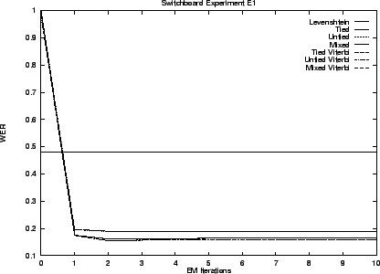 cost of selecting
a component is usually very small compared to the total
 of the mixture's value. For this reason they
operate as a stochastic or gate of sorts. That is,
the probability is high if that of any component is.
One use of mixtures is to combine models of increasing complexity as a strategy to combat overtraining. We implement a particular simple case in which our tied and untied model forms are combined by a uniform fixed mixture.
Another richer use of mixtures uses them to capture possible modality in the process that generates surface phonetic forms from lexical forms. Different speaker types might well exhibit very different transductive characteristics and a stronger overall model will result if they are separately modeled and combined as a mixture. Different transducers might also be trained for very different corpa and then combined in a mixture. There are many other possibilities and the general approach represents an interesting area for future work. In our experiments the mixing coefficients are fixed and uniform, but they might have been optimized using withheld training data [FJM80].
During training we do not know a priori which lexical phonetic form gave rise to the surface form observed. A feature of our hidden stochastic mixture approach is that all possibilities are considered, each reinforced in proportion to the model's a posteriori estimate that it generated the observation. During recognition, contributions from all possibilities are combined within a proper probabilistic framework.
A simpler ad hoc approach reinforces all possibilities equally during learning. During recognition a simple nearest neighbor approach is taken. That is, the least distant lexical phonetic form determines the decision.
All experiments were performed for both strategies to support comparison.
We begin by presenting results for our hidden stochastic mixture approach to the problem - our preferred solution. Results for the ad hoc approach are presented last. Table 3.5 summarizes these results. The error rates shown are the best observed during training. That is, as though an oracle told us when to stop performing EM iterations.
Notice that the transduction distances exhibit error rates less than one third that of Levenshtein distance. As we anticipated the Viterbi and stochastic edit distance behave similarly. The untied model is superior in all cases.
The graphs that follow give performance throughout training. The initial performance of transduction distance is poor because training starts with a uniform model.
|
|
|
|
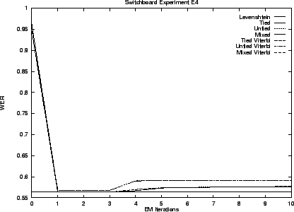
We now turn to results from our ad hoc approach described earlier. It is apparent that trained transduction distances perform poorly relative to simple Levenshtein distance - especially in settings E3 and E4. None of the transduction distances is significantly better than the untrained Levenshtein distance in this approach.
Despite its simplicity this approach is conceptually unsatisfactory because it frequently trains the transducer with unrelated pairs, diluting the effectiveness of learning. Indeed the performance of the trained edit distances is not very different from that of Levenshtein distance. Our results make clear that the added complexity of our preferred stochastic mixture approach is not just conceptually superior, but is empirically warranted.
| ||||||||||||||||||||||||||||||||||||||||||||||||
The graphs that follow show performance during training.
|
|
|
|
|
An immediate opportunity exists to improve performance by adding a higher order language model to the system. Mixtures of untied transducers also may help given additional training data.
But our positive results for experiment E3 suggest perhaps the most interesting next step: replace the manual transcript labeling step, with an automatic process - even if the phonemes it recognizes are somewhat noisy and do not correspond perfectly with standard categories. Then enhance the transductive model to include memory, that context sensitivity.
Even this is just one step towards a yet more interesting
objective: demonstrating that one may bridge the entire
![]() gap within the framework of stochastic
transduction, learning if necessary one or more hidden
languages analogous to the artificial phonetic language
invented by human linguists.
gap within the framework of stochastic
transduction, learning if necessary one or more hidden
languages analogous to the artificial phonetic language
invented by human linguists.
In section 3.2 we made the simplifying
assumption that ![]() is optimized by instead
optimizing the joint transduction probability
is optimized by instead
optimizing the joint transduction probability ![]() .
Moreover we remarked that our experiments did not in
fact exactly implement the framework described.
.
Moreover we remarked that our experiments did not in
fact exactly implement the framework described.
This section clarifies these issues by providing an alternative formulation for which no such assumption is necessary. Its implementation and evaluation is, however, left to future work.
The model derivation of section 3.2 may be
altered so that the joint probability ![]() is
factored instead as
is
factored instead as
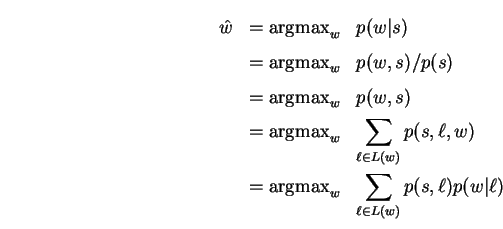 resulting in the revised model and decision rule:
The virtue of this alteration is that the joint transduction
probability ![]() is now used directly.
is now used directly.
Another issue surrounds this transduction probability. As we've implemented it, it does not directly correspond to a generative model for finite strings. But as discussed in section 2.5.1 of chapter 2, it is possible to compute honest probabilities that are conditioned on string lengths. Combining such a model with one for the lengths leads to the generative model required to neaten the conceptual framework of this chapter.