Data Structures and Algorithms for Nearest Neighbor Search in General Metric Spaces

Peter N. Yianilos
NEC Resarch Institute

Abstract:

We consider the computational problem of finding nearest neighbors in general metric spaces. Of particular interest are spaces that may not be conveniently embedded or approximated in Euclidian space, or where the dimensionality of a Euclidian representation is very high.

Also relevant are high-dimensional Euclidian settings in which the distribution of data is in some sense of lower dimension and embedded in the space.

The vp-tree (vantage point tree) is introduced in several forms, together with associated algorithms, as an improved method for these difficult search problems. Tree construction executes in $O(n \log(n))$ time, and search is under certain circumstances and in the limit, $O(\log(n))$ expected time.

The theoretical basis for this approach is developed and the results of several experiments are reported. In Euclidian cases, kd-tree performance is compared.

Keywords: Metric Space, Nearest Neighbor, Computational Geometry, Associative Memory, Randomized Methods, Pattern Recognition, Clustering.

Introduction.

Nearest neighbor analysis is a well established technique for non-parametric density estimation, pattern recognition, memory-based reasoning, and vector quantization. It is also highly intuitive notion that seems to correspond in some way with the kind of inexact associative recall that is clearly a component of biological intelligence.

One useful abstraction of nearness is provided by the classical notion of a mathematical metric space [1]. Euclidian $n$-space is but one example of a metric space.

The Nearest Neighbor field includes the study of decision making and learning based on neighborhoods, the underlying metrics and spaces, and the matter of computing/searching for the neighborhood about a point. See [2] for a recent survey. Our focus is on search, and, for simplicity, on locating any single nearest neighbor.

Given a fixed finite subset of the space and calling it the database, our task is then to locate for each new query drawn from the space, a database element nearest to it.

As the database is finite, we might search by considering every member. But in a somewhat analogous setting, binary search can locate a queries position within a finite ordered database while considering only $\log(n)$ elements. Moreover, binary search proceeds given only ordinal knowledge. I.e., it doesn't matter what the database objects are.

So while the notions of ordering and metric-distance are only loosely analogous, we are nevertheless motivated to look for improved search methods that depend only on the information received through metric evaluation.

Now binary search presumes that the database has been sorted - an $n \log(n)$ process. We then seek to organize our database in as much time so that under some circumstances, logarithmic time search is possible.

We introduce the vp-tree (vantage point tree) in several forms as one solution. This data structure and the algorithms to build and search it were first discovered and implemented by the author during 1986-87¹ in conjunction with the development of improved retrieval techniques relating to the PF474 device [3]. Motivation was provided by the fact that this chip's notion of string distance is non-Euclidian. Here elements of the metric space are strings, E.g., a database of city names and associated postal codes. This early work was described in [4].

Independently, Uhlmann has reported the same basic structure [5,6] calling it a metric tree.

There is a sizable Nearest Neighbor Search literature, and the vp-tree should properly be viewed as related to and descended from many earlier contributions which we now proceed to summarize.

Burkhard and Keller in [7] present three file structures for nearest neighbor retrieval. All three involve picking distinguished elements, and structuring according to distance from these members. Their techniques are coordinate free. The data structures amount to multi-way trees corresponding to integral valued metrics only.

Fukunaga in [8,9] exploits the triangle inequality to reduce distance computations searching a hierarchical decomposition of Euclidian Space. His methods are restricted to a Euclidian setting only by his use of a computed mean point for each subset. However this is not an essential component of his approach - at least conceptually. He recursively employs standard clustering [10] techniques to effect the decomposition and then branch-and-bound searches the resulting data structure. During search, the triangle inequality implies that a cluster need not be explored if the query is far enough outside of it. While exploring a cluster at the lowest level, Fukunaga further points out that the triangle inequality may be used to eliminate additional distance computations. A key point apparently overlooked, is that when the query is well inside of a cluster, the exterior need not be searched.

Collections of graphs are considered in [11] as an abstract metric space with a metric assuming discrete values only. This work is thus highly related to the constructions of [7]. In their concluding remarks the authors correctly anticipate generalization to more continuous settings such as ${\mathbb{R}}^n$.

The kd-tree of Friedman and Bentley [12,13,14,15] has emerged as a useful tool in Euclidian spaces of moderate dimension. Improvements relating to high-dimensional settings, distribution adaptation, and incremental searches, are described in [16], [17], and [18] respectively.

A kd-tree is built by recursively bisecting the database using single coordinate position cuts. For a given coordinate, the database is cut at the median of the distribution generated by projection onto that coordinate. An optimized kd-tree results by choosing the cutting coordinate to be that whose distribution exhibits the most spread.

In addition to various vp-tree forms, we have implemented optimized kd-tree software so that experimental comparisons can be made operating on identical spaces and given identical query sequences.

Like the kd-tree, each vp-tree node cuts/divides the space. But rather than using coordinate values, a vp-tree node employs distance from a selected vantage point. Near points make up the left/inside subspace while the right/outside subspace consists of far points. Proceeding recursively, a binary tree is formed. Each of its nodes identifies a vantage point, and for its children (left/right), the node contains bounds of their associated subspace as seen by the vantage point. Other forms of the vp-tree include additional subspace bounds and may employ buckets near leaf level.

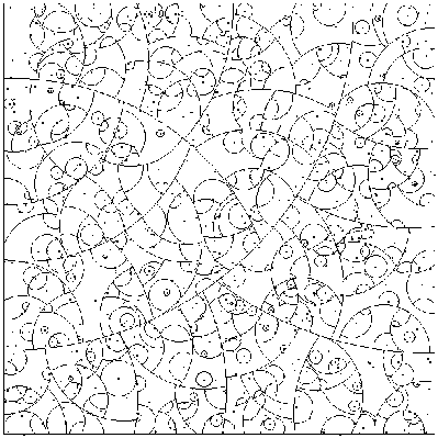
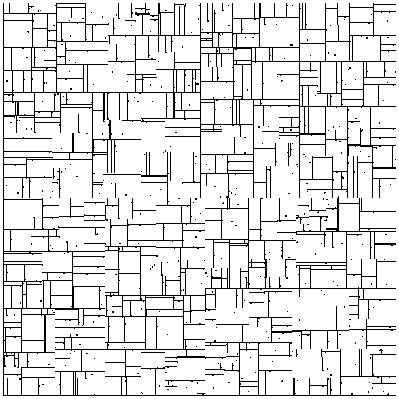
To build these structures, the metric space is decomposed using large spherical cuts centered in a sense at elements near the corners of the space. This contrasts with the coordinate aligned hyperplanar cuts of the kd-tree (See Figures 1 & 2), and the use of computed Euclidian cluster centroids in [8]. Randomized algorithms for vp-tree construction execute in $O(n \cdot \log(n))$ time and the resulting tree occupies linear space.

Figure 1: vp-tree decomposition

Figure 2: kd-tree decomposition

For completeness, early work dealing with two special cases should be mentioned. Retrieval of similar binary keys is considered by Rivest in [19] and the $L_\infty$ (max) metric setting is the focus of [20].

More recently, the Voronoi digram [21] has provided a useful tool in low- dimensional Euclidian settings - and the overall field and outlook of Computational Geometry has yielded many interesting results such as those of [22,23,24,25] and earlier [26].

Unfortunately neither the kd-tree, or the constructions of computational geometry, seem to provide a practical solution for high dimensions. As dimension increases, the kd-tree soon visits nearly every database element while other constructions rapidly consume storage space.

Furthermore, even if the database is in some sense of only moderately high dimension, it may not be possible or convenient to find or implement a dimension reducing transformation. So it is important that we develop techniques that can deal with raw untransformed data, and exhibit behavior as close as possible to intrinsic rather than representational dimension.

So despite considerable progress for Euclidian space, the development of more general techniques is important; not just because of the problems with high dimension, but also because there is no a priori reason to believe that all or even most useful metrics are Euclidian.

In the sections that follow we will consider a probabilistic formulation of the problem and obtain certain theoretical results, present the algorithms and data structures for the vp-tree in several forms, and report on a number of experiments. These experiments include Euclidian cases with side-by-side kd-tree comparisons, non-Euclidian spaces, and the difficult real-world problem of image fragment retrieval. Here fragments as large as $50 \times 50$ pixels are treated corresponding to representational dimension $2,500$.

Theoretical Insight and Basic Results.

In this section we develop a simple but fairly general result which says that under certain circumstances, one may organize a database so that expected search time is logarithmic. It should be thought of as justifying in the limit the algorithms and data structures presented later. Only elementary concepts from General Topology and Measure/Probability Theory are employed.

Notation.

Given a metric space $({\cal S},d)$ and some finite subset ${\cal S}_D \subset {\cal S}$ representing the database against which nearest neighbor queries are to be made, our objective is to somehow organize ${\cal S}_D$ so that nearest neighbors may be more efficiently located.

For a query $q \in {\cal S}$, the nearest neighbor problem then consists of finding a single minimally distant member of ${\cal S}_D$. We may write $\mbox{NN}(q,{\cal S}_D)$ to stand for this operation where the space may be omitted for brevity.

Now the element nearest to $q$ may be quite far, and for a particular problem it may be reasonable to impose a distance threshold $\tau$, at or beyond which one is uninterested in the existence of neighbors. Also observe that while computing $\mbox{NN}(q)$, one may by reduce $\tau$ as ever nearer neighbors are encountered. We write $\mbox{NN}\vert _\tau (q,{\cal S}_D)$ to denote this important notion of $\tau$ restricted search.

Next we will assume that the range of the space's distance distance function is $[0,1]$. Since any metric's range may be compressed to this interval without affecting the nearest-neighbor relation², this restriction may be made without loss of generality³.

Vantage Points.

Each element of a metric space has in a sense a perspective on the entire space; formed by considering its distances to every other element. This perspective need not however contain any information. Consider the pathological case of the discrete metric in which the distance between any pair of distinct points is one. Here, full-space search is unavoidable. However, to the extent that information is present, we will see that nearest neighbor search may benefit.

We begin by formalizing this notion of perspective and defining a related pseudo-distance function:

Definition 1  

Let $({\cal S},d)$ be a $[0,1]$ bounded metric space. Given a distinguished element $p \in {\cal S}$, we make the following definitions for all $a,b \in {\cal S}$:

1. $\Pi_p: {\cal S}\rightarrow [0,1]$ is given by: $\Pi_p(a) = d(a,p)$.

2. $d_p: {\cal S}\times {\cal S}\rightarrow [0,1]$ is given by: $d_p(a,b) = \vert\Pi_p(a) - \Pi_p(b)\vert = \vert d(a,p) - d(b,p)\vert$.

Function $\Pi_p$ is best thought of as a projection of ${\cal S}$ into $[0,1]$, from the perspective of $p$. I.e. it is ${\cal S}$ as seen by $p$, via $d$. Function $d_p$ is not in general a metric since if $a$ and $b$ are distinct but equidistant from $p$, $d_p(a,b)=0$. It is however a clearly symmetric function and satisfies the triangle inequality, making it a pseudo-metric.

Now since $d$ is a metric we may rely on symmetry and the triangle inequality to arrive at:

$$d(a,b) \geq \vert d(a,p) - d(b,p)\vert = d_p(a,b)$$

Hence, distances shrink when measured by $d_p$ so that $d$ in a sense dominates it. One useful consequence of this behavior is given by the following obvious implication:

$$d_p(a,b) \geq \tau \Rightarrow d(a,b) \geq \tau$$ (1)

So if during a search we've already encountered a database element $x$ at distance $\tau$ from $q$, then as our search progresses, we need not consider any element for which $d_p(q,x) \geq \tau$. Thus, in the absence of coordinates or Euclidian structure, we can begin to see how query's distance to a distinguished vantage point may be exploited to effectively direct and limit the search.

For some $p \in {\cal S}_D$ consider now the image $\Pi _p({\cal S}_D)$ of ${\cal S}_D$ in $[0,1]$. Next denote by $\mu$ the median of $\Pi _p({\cal S}_D)$ thus dividing $[0,1]$ into $[0,\mu)$ and $[\mu,1]$. The first of these intervals contains points from the inside the sphere $S(p,\mu)$, while the second consists of points from outside and on the surface. We denote the inverse images of these $S_{p_L}$ and $S_{p_R}$ respectively; and imagine that ${\cal S}_D$ is divided in this way into left and right subspaces.

Now $N_L = \vert S_{p_L}\vert$ counts the points of ${\cal S}_D$ mapped left to $[0,\mu)$, while $N_R = \vert S_{p_R}\vert$ counts those sent right to $[\mu,1]$. We can say little in general about the comparative sizes of $N_L$ and $N_R$ since nothing has been assumed about the nature of the metric space. In particular if there are many points of ${\cal S}_D$ exactly distance $\mu$ from $p$, then $N_R$ may be much larger than $N_L$.

But if spheres in $({\cal S}_D,\mu)$ typically have on their surface relatively few members of ${\cal S}_D$, then we can say that $N_L \approx N_R$, i.e, we have partitioned ${\cal S}_D$ into two subsets of roughly equal size.

Now suppose for a given $q$, that our objective is $\mbox{NN}\vert _\tau (q)$, and that $\Pi_p(q) \geq \mu + \tau$. Then it follows from EQ- 1 that $S_{p_L}$ may be excluded from consideration. Similarly if $\Pi_p(q) \leq \mu - \tau$, we may ignore $S_{p_R}$. In both cases then, roughly half the space is excluded from consideration. Thus, the information gleaned from a single point's perspective is sometimes sufficient to significantly prune the search. However if $\mu-\tau < \Pi_p(q) < \mu+\tau$, then no such reduction is possible.

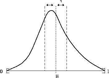
So it is clear that our ability to prune is dependent on a fortuitous choice of $p$ and $q$, on $\tau$, and on our ability to choose $N_L \approx N_R$. We will succeed to the extent that it is improbable that $\Pi_p(q) \in (\mu-\tau,\mu+\tau)$ (Figure 3).

If our probability distribution is in some sense nice (see §2.3), then we can make this probability approach zero as $\tau$ does. So that for $\tau$ sufficiently small, we will with high probability exclude approximately half of the space from consideration.

Figure 3: A continuous rendering of the density of $\Pi _p({\cal S}_D)$ in [0,1] - and a $\tau$ neighborhood of median $\mu$

It is easy now to see how we may recursively proceed to form a binary tree. This then forms the most basic vp-tree. Specific construction and search algorithms are presented in §3.

A Probabilistic Viewpoint.

Since individual instances of finite metric spaces (databases) may be pathological for nearest neighbor search, we are led to formulate the problem in probabilistic terms and seek expected time results.

We therefore define probability measure $P$ which we assume reflects the distribution from which both database elements and queries are drawn⁴. It is worthwhile noting that the arguments that follow may be generalized to deal with separate distributions.

Now from EQ- 1 it is clear that mapping $\Pi_p$ is uniformly continuous, from which it follows that the inverse images of any point or interval (whether open, closed, or half-open) must have defined probability.

Thus, given some such point or interval $X$, we may for the sake of notational simplicity refer to $P(X)$ which is understood to mean $P(\Pi_p^{-1}(X))$. So if $x \in [0,1]$, then $P(x)$ is the probability of the surface of sphere $S(p,x)$.

Now in the case of the discrete metric, there is about every point a spherical surface of probability one. This is in stark contrast to Euclidian settings where any volume related probability measure results in zero probability spherical surfaces. Remembering that the discrete metric is pathological to nearest neighbor schemes, we are led to consider metrics which share this property.

Definition 2  

Let $({\cal S}, d, P)$ be a metric space with associated probability measure $P$, the combination is said to have the ZPS (Zero Probability Spheres) property if and only if: $P(S_s(x,r)) = 0, \forall x \in {\cal S}, r \geq 0$, where $S_s(x,r) = \{y \in {\cal S}\vert d(y,x) = r\}$.

The discrete metric is thus excluded along with many other cases. This is however a very strong condition. We assume it for simplicity's sake but comment that there are several ways to weaken it while preserving the essence of the arguments that follow.

Basic Results.

The probability of a countable intersection of nested sets, is just the limit of the individual probabilities. This and ZPS then imply that about any $x \in [0,1]$, there exists an interval of arbitrarily small probability. Nothing more than this basic observation is necessary to establish the two simple theorems that follow. It is however worth remarking that uniform convergence to zero probability can be established. I.e., given $\epsilon > 0$, there exists $N$ sufficiently large, so that every interval of the canonical $[0,1]$ $N$-partitioning, has probability less than $\epsilon$.

We now make more rigorous our earlier comments regarding procedures for recursive space bisection.

Theorem 1   Let $({\cal S}, d, P)$, be a $[0,1]$ bounded metric space with the ZPS property under probability measure $P$. Then except for cases of probability zero, every size $n$ database ${\cal S}_D\subseteq {\cal S}$ drawn from $P$, may be organized into a binary tree; so that given $M > 1$, and queries `$q$' drawn from $P$, $\exists$ $\tau > 0$ such that $\mbox{NN}\vert _\tau (q,{\cal S}_D)$ may be computed using at most $M \cdot \lfloor \log_2(n)+1\rfloor$ metric evaluations on an expected basis.

proof: Let $d = \lfloor \log_2(n)+1 \rfloor$ and if $n < 2^d-1$ draw additional elements until equality.

Pick some $p_1 \in {\cal S}_D$ and consider $\Pi_p({\cal S}_D-\{p_1\})$. Set value $\mu_1$ so that equally many image points are to its left and right. Continue recursively bisecting the space - forming a binary tree and establishing $\mu_i$ for each non-leaf element of ${\cal S}_D$. By ZPS this is almost always possible (failure probability zero).

Define $\epsilon = (M^{1/(d-1)} - 1)/2$ so $M = (1+2\epsilon)^{d-1}$.

Associate with $p_1$ values $\psi_{L_1} = P([0,\mu_1))$ and $\psi_{R_1} = P([\mu_1,1])$. Now by our earlier comments we may choose $\tau_1$ such that $P([\mu_1-\tau_1,\mu_1+\tau_1]) < \epsilon$.

In what follows we will proceed recursively to associate $\psi$ and $\tau$ values to each non-leaf node.

The root's probability function is just $P$. We define that of its left child to be essentially $P_L=P\vert[0,\mu_1+\tau_1)$ but more formally $P_L(X) = P(X \cap \Pi_{p_1}^{-1}([0,\mu_1+\tau_1)))/P([0,\mu_1+\tau_1))$.

To understand this observe that $\mbox{NN}\vert _{\tau_1}$ search will explore leftward only if $\Pi(q) \in [0,\mu_1+\tau_1)$. An alternative view is that the left subtree is only concerned with the subspace $\Pi_{p_1}^{-1}([0,\mu_1+\tau_1))$ and sees it as the entire space. In a similar way we associate a new probability function with the right child. Now it must be noted that these modified functions remain probability measures, and inherit ZPS.

Having done this, $\psi$ and $\tau$ values may be associated with the left and right child. This enables the process to continue down the tree until all non-leaf nodes have values. Finally set $\tau = \min \tau_i$.

For a query $q$ drawn by $P$, We compute $\mbox{NN}\vert _\tau (q)$ starting at the root. Thus a single metric evaluation is always performed. Then with probability of no more than $\psi_{L_1}+\epsilon$, we will be required to explore leftward. The probability of rightward exploration is similarly bounded by $\psi_{R_1}+\epsilon$. In both cases the subtrees will see the query as random within their subspaces of interest.

If leaf level is reached, a single evaluation is always performed. It then follows that the overall cost (metric evaluations) of the search is on an expected basis is the value $F(d)$ where $F(1)=1$ and $F(i)=1 + (1+2\epsilon) F(i-1)$. This recursion evaluates to $F(d)=\sum_0^{d-1} (1+2\epsilon)^i$ which is bounded above by $(1+2\epsilon)^{d-1} d = M \cdot \lfloor \log_2(n)+1 \rfloor$ $\Box$

$\;\Box$

A result similar in flavor may be proven in which a tree is built and used to classify additional members of the space so that all buckets (leaf levels) have equal probability. Each of these leaves then correspond to a subspace of the metric space and we have in effect then equipartitioned the space with respect to the probability distribution. This is analogous to vector quantization in Euclidian space. Thinking of the root-leaf path as a binary code, we might also interpret it as metric space hashing.

Theorem 2   Let $({\cal S}, d, P)$, be a $[0,1]$ bounded metric space with the ZPS property under probability measure $P$. Then for any fixed database size $n$, and $M > 1$, $\exists$ $\tau > 0$ such that we may compute $\mbox{NN}\vert _\tau (q,{\cal S}_D)$ with at most $M \cdot \lceil \log_2(n) + 1\rceil$ expected metric evaluations; as databases ${\cal S}_D\subseteq {\cal S}$ and queries `$q$' are drawn from $P$.

proof: For brevity's sake assume $n$ is a power of 2. As in the previous theorem we will build a binary tree. Before we were forced to bisect a particular finite database at each level so that in general $\psi_L \neq \psi_R$. Here we begin by building a balanced binary tree so that its initial $\lceil \log_2(n) + 1 \rceil$ levels have $\psi_{L_i} = \psi_{R_i} = 1/2$. We may do this by picking for the root an arbitrary element, then setting the root's $\mu$ so that $\psi_L=\psi_R$. Having done this we may pick a vantage point for the left and right children from the associated subspaces and proceed recursively to the required depth.

Observe that the leaf level subspaces have equal probability of $1/n$. As for theorem- 1 we may find $\tau$ for this tree so that we expect to visit at most $M \cdot \lceil \log_2(n) + 1\rceil$ nodes. So clearly no more than this number of leaf nodes will be visited on an expected basis.

Now each element of a particular drawn database may be classified and then attached to this tree by first identifying which of the $1/n$ leaf partitions it belongs to, and adding it to an initially empty list rooted at and replacing the corresponding leaf node. The expected size of each list is clearly one. So the final expected number of metric evaluations remains $M \cdot \lceil \log_2(n) + 1\rceil$. $\Box$

$\;\Box$

These theorems describe binary constructions to motivate the algorithms and experiments which follow; but higher degree trees may be built by further partitioning $[0,1]$. In the extreme case the root has degree $n$ and only three metric evaluations are expected. As a practical matter however, the $\tau$ values necessary to approach even $\log_2(n)$ search are so small as to be of little practical value. So the basic theorems presented are best thought of as existence results which establish a theoretical foundation while motivating algorithm development.

Corners of the Space.

Now it is fairly clear that we'd like $\tau$ as large as possible; and its value depends on $\Pi_p$ and hence on $p$. This then suggests that some elements of the space may be better vantage points than others. We are thus lead to consider the problem of selecting a vantage point.

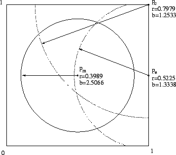
As an example consider the unit square with uniform probability distribution. Here we must choose $\mu$ so that two regions of area $0.5$ result. Three natural choices for $p$ consist of the square's midpoint (denoted $p_m$), a corner (denoted $p_c$), and the midpoint of an edge (denoted $p_e$). These along with their associated division boundaries are illustrated in Figure 4.

Figure 4: Natural choices for $p$ to divide the unit square

To choose among them, notice that for small $\tau$ the length of the boundary will be proportional in the limit to the probability that no pruning takes place. Thus minimizing these boundary lengths (denoted $b$ in the figure) is the obvious strategy.

Observe that $p_m$ is by far the worst choice as its boundary length is double that of $p_c$. Choice $p_e$ is also much better than $p_m$, but not quite as good as $p_c$. It is interesting to note that from a traditional clustering viewpoint, $p_m$ is the natural centroid. But we have seen that it is far from the best choice. From this example we draw the intuition that points near the corners of the space make the best vantage points. (See again the vp-tree decomposition of Figure- 1).

These simple results then suggest a strategy for vantage point selection, and given a particular distribution, provide a framework for drawing more conclusions. The ZPS distribution restriction is key to achieving them; and our overall outlook in which finite cases are imagined to be drawn from a larger more continuous space, distinguishes in part this work from the discrete distance setting of [7,11].

Set Perspectives.

We have seen that a single distinguished element $p$, induces a pseudo-metric $d_p$, which is always dominated by $d$. More generally, we observe that each size $n$ finite subset $P$ of a metric space, considered as vantage points, induces a natural mapping into Euclidian n-space. I.e. the $i$-th coordinate of the image of $x$, is just $\Pi_{p_i}(x)$.

Under $L_\infty$ then, distances in the Euclidian range space are always dominated by distances in the domain. This amounts to Euclidian approximation of the original metric. This mapping and elementary observation will help us later define enhanced forms of the vp-tree.

Algorithms and Data Structures.

The Simplest vp-tree.

We begin by presenting a simple algorithm for vp-tree construction. The root corresponds to the entire space. Its distinguished vantage point then splits the space into left and right subspaces corresponding to the root's left and right tree descendants. Similarly, each node is thought of as corresponding to an ever smaller subset of the database.

An optimized tree results because function Select_vp endevours to pick better than random vantage points. Replacing it with a simple random selection generates a valid and effective tree; but experiments have shown that some effort towards making better choices, results in non-trivial search-time savings. Our algorithm constructs a set of vantage point candidates by random sampling, and then evaluates each of them. Evaluation is accomplished by extracting another sample, from which the median of $\Pi_p({\cal S})$, and a corresponding moment are estimated. Finally, based on these statistical images, the candidate with the largest moment is chosen. Given constant size samples, execution time is $O(n \log(n))$. Our experimental implementation includes several sampling and evaluation parameters.

Algorithm 1   Given set S of metric space elements; returns pointer to the root of an optimized vp-tree.

function Make_vp_tree(S)

if $S = \emptyset$ then return $\emptyset$

new(node);

node$\uparrow$.p $:=$ Select_vp(S);

node$\uparrow$.mu $:=$ $\mbox{Median}_{s \in S}$ $d(p,s)$;

L $:=$ $\{s \in {\cal S}\! - \!\{p\} \vert d(p,s) < \mbox{mu}\}$; R $:=$ $\{s \in {\cal S}\! - \!\{p\} \vert d(p,s) \geq \mbox{mu}\}$;

node$\uparrow$.left $:=$ Make_vp_tree(L); node$\uparrow$.right $:=$ Make_vp_tree(R);

return node;

function Select_vp(S)

P $:=$ Random sample of S;

best_spread $:=$ 0;

for $p \in P$

D $:=$ Random sample of S;

mu $:=$ $\mbox{Median}_{d \in D}$ $d(p,d)$;

spread $:=$ $\mbox{2nd-Moment}_{d \in D}$ $(d(p,d)-\mbox{mu})$;

if spread $>$ best_spread best_spread $:=$ spread; best_p $:=$ p;

return best_p;

In the simple construction above, only mu is retained in a node to describe the metric relationship of the left/right subspaces to the node's vantage point. At the expense of storage space, one may retain instead four values representing lower/upper bounds of each subspace as seen by the vantage point. It is this form of tree that is actually used in the experiments we later report.

The $\mbox{vp}^{\mbox{s}}$-tree.

Now notice that in the course of execution, an element of $S$ is compared with the vantage point belonging to each of its ancestors in the tree. This information is also not captured in the simple tree described above. Retaining it in a particular way results in a $\mbox{vp}^{\mbox{\footnotesize s}}$-tree - the construction of which we now describe.

The central working structure employed consists of a database element identifier `id', and a list `hist' of distances from the item to each vantage point tracing back to the root. A list of these structures is initialized from the entire database, with the history set to null. The algorithm then recursively splits the list into two lists $L$ and $R$, while adding to the history of each item. Each resulting tree node then contains a list `bnds' giving lower and upper bounds (a range interval) for its corresponding subspace as seen by each ancestral vantage point.

Execution time remains $O(n \log(n))$. Assuming fixed precision is used to represent the bounds, the tree occupies linear space. But this is an asymptotic statement, and over the practical range of $n$, and given fixed machine word sizes, the space is better described by $O(n \log(n))$.

Algorithm 2   Given set S of metric space elements; returns pointer to the root of an optimized $\mbox{vp}^{\mbox{\footnotesize s}}$-tree.

function Make_vps_tree(S)

list = $\emptyset$;

for $s \in S$ new(item); item$\uparrow$.id $:=$ $\uparrow$$s$; item$\uparrow$.hist $:=$ $\emptyset$; add item to list;

return Recurse_vps_tree(list);

function Recurse_vps_tree(list)

if list $= \emptyset$ then return $\emptyset$

new(node); node$\uparrow$.p $:=$ Select_vp(list);

delete node$\uparrow$.p from list;

for item $\in$ list append d(p,item$\uparrow$.id) to item$\uparrow$.hist;

mu $:=$ $\mbox{Median}_{\mbox{item} \in \mbox{list}}$ tail(item$\uparrow$.hist);

L $:=$ $\emptyset$; R $:=$ $\emptyset$;

for item $\in$ list if tail(item$\uparrow$.hist) $< \mbox{mu}$ then add item to L, delete from list; else add item to R, delete from list;

node$\uparrow$.left $:=$ Recurse_vps_tree(L); node$\uparrow$.right $:=$ Recurse_vps_tree(R);

node$\uparrow$.bnds $:=$ Merge(node$\uparrow$.left$\uparrow$.bnds, node$\uparrow$.right$\uparrow$.bnds,node$\uparrow$.p$\uparrow$.hist);

return node;

function Merge(range_list1,range_list2,value_list) ``The two range lists are combined with the value list to yield a single range list which is returned.''⁵

There's no guaranty that these algorithms build a balanced tree⁷ - for in practice, the ZPS assumption may not hold. Furthermore, even if it does, we may draw a rather pathological database. So in the end, the balance achieved is problem dependent.

The $\mbox{vp}^{\mbox{sb}}$-tree.

Our constructions so far have involved a single node structure. We now consider one way to form buckets of leaves in order to save space while preserving the notion of ancestral history present in the $\mbox{vp}^{\mbox{\footnotesize s}}$-tree. Buckets are formed by collapsing subtrees near leaf level into a flat structure. Each bucket contains say $n_b$ element records. Each record must specify an id, and in addition holds distance entries for every ancestor. We call the resulting structure a $\mbox{vp}^{\mbox{\footnotesize sb}}$-tree. In our implementation the bucket distance values are quantized so as to occupy only 2-bytes.

One may think of these vectors of distances, as the image of an element under the set perspective mapping defined by the ordered set of its ancestors. (§2.6)

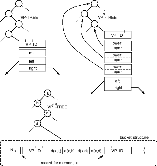
The data structures corresponding to these three tree types are depicted in Figure- 5. Database elements are represented by a 4-byte integer, real values by a 4-byte float, and bucket distances by a 2-byte integer. These correspond closely to our experimental implementation; except that the $\mbox{vp}^{\mbox{\footnotesize }}$-tree we implement contains subspace bounds rather than the single value mu.

Figure: Sample 32-bit machine data structure implementations for the most basic vp-tree, the $\mbox{vp}^{\mbox{s}}$-tree, and the $\mbox{vp}^{\mbox{sb}}$-tree.

Searching the tree.

We present a single search algorithm which describes search in a vp-tree where a node contains subspace bounds for each child. The algorithm is easily generalized to the other tree forms. It is a straightforward recursive branch-and-bound tree search in which variable tau keeps track of the closest neighbor yet encountered. Subtrees are then pruned when the metric information stored in the tree suffices to prove that further consideration is futile. I.e., cannot yield a strictly closer neighbor.

Algorithm 3   Called with query `q' and the root of a vp-tree; returns the `id' of a nearest neighbor in global variable `best'. Before calling, global variable `tau' is set to the desired search radius and `best' should be set to $\emptyset$. Setting tau to 1 then searches without constraint. On return `tau' is the distance to `best'. We denote by $I_L$ the open interval whose left endpoint is n$\uparrow$.left_bnd[low]-tau and right endpoint is n$\uparrow$.left_bnd[high]+tau. Open interval $I_R$ is defined similarly.

procedure Search(n)

if n $= \emptyset$ then return ;

x $:=$ d(q,n$\uparrow$.id);

if x $<$ tau then tau $:=$ x; best $:=$ n$\uparrow$.id;

middle $:=$ (n$\uparrow$.left_bnd[high] + n$\uparrow$.right_bnd[low])/2;

if x $<$ middle then if x $\in I_L$ then Search(n$\uparrow$.left); if x $\in I_R$ then Search(n$\uparrow$.right); else if x $\in I_R$ then Search(n$\uparrow$.right); if x $\in I_L$ then Search(n$\uparrow$.left);

Notice that the order of exploration is determined by comparison with the middle value computed. This is properly viewed as a heuristic. In high dimensions this may not be the best choice and branching order represents an interesting area for future work.

Actual databases, particularly those consisting of signals or images, frequently contain large clusters of very similar items. In these cases one may find that search rapidly locates a very near neighbor, and then performs much more work which yields only a very slightly nearer item. Because of this problem, our implementation includes an error tolerance setting which in effect narrows intervals $I_L$ and $I_R$. E.g. Given tolerance 0.01, the procedure will return a neighbor which is guaranteed to be at most 0.01 more distant from the query than its true nearest neighbor.

Now having summarized and sketched our algorithms and data structures, we turn to experimental results.

Selected Experimental Results.

A modular software system was built with plug-in metric spaces and search routines. Two basic metric space settings were implemented: hypercubes, and image fragments. Both support various metrics including the standard Minkowski family.

Hypercubes.

We very nearly reproduce certain of the experimental settings from [13] and use them to begin our process of evaluation. Hypercubes of increasing dimension are first considered, each containing a database consisting of 8,192 coordinate-wise normally distributed pseudorandom points.

The vp-tree⁸ and kd-tree are compared for the $L_1$, $L_2$, and $L_\infty$ metrics as dimension ranges from 2 to 14. Since interior vp-tree nodes contain data elements while the kd-tree contains data elements at its leaf level only, we use total nodes visited to measure complexity. The resulting statistics were observed to agree well with actual CPU time used.

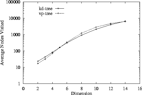
Figure 6 demonstrates the remarkable agreement between these two methods for the $L_2$ metric. Similar agreement is found for the $L_\infty$ metric, while for $L_1$, the vp-tree maintains a small constant advantage. Detailed examination of the results does however reveal one qualitative difference which increases with dimension. By dimension 14, the kd-tree visits roughly $5.7$ times as many nodes under $L_1$ versus $L_\infty$. The ratio for vp-tree search is only $1.7$. This suggests that vp-tree performance may be flatter with respect to choice of metric.

Figure 6: Search Cost vs. Dimension Comparison For $L_2$ Metric and Based on Nodes Visited

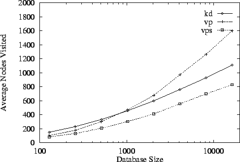
If dimension is fixed and database size grows, we expect and find asymptotically logarithmic growth in search time. For dimension 8 (Figure 7), kd-tree performance is in the limit between that of the vps-tree and vp-tree. Examining CPU time, the same is true although the differences are smaller. In dimensions 2 and 4, the performance ordering from best to worst is vps-tree, vp-tree, then kd-tree for all database sizes.

Figure 7: Search Cost vs. Database Size - Dimension 8

The kd-tree does however eventually catch up in this random hypercube environment. By dimension 12 for example, it visits fewer nodes than vps-tree search once database size grows beyond $30,000$. By this point however, neither perform very well - visiting roughly $25\%$ of the nodes.

So despite their ignorance of the coordinate structure of the space, and randomized construction, vp-trees compare well in this setting with the kd-tree.

Comparisons with the experiments of [8] are more difficult because leaf level buckets are employed. Nevertheless, based purely on metric evaluations, the kd-tree and vp/ $\mbox{vp}^{\mbox{\footnotesize s}}$-tree methods produce superior results.

Random Linear Embedding.

As a simple embedding model, we construct random linear rotation matrices which correspond to isometric embeddings of ${\mathbb{R}}^m$ into ${\mathbb{R}}^n$ where $n > m$.

Pseudorandom databases are then drawn in a coordinate-wise uniform fashion within ${\mathbb{R}}^m$ and mapped to the longer vectors of ${\mathbb{R}}^n$.

To study this setting we define three types of query distribution - all pseudo-random but confined to different subspaces:

T1:

Drawn in ${\mathbb{R}}^m$ and then mapped to ${\mathbb{R}}^n$.

T2:

Drawn in ${\mathbb{R}}^n$.

T3:

Drawn in ${\mathbb{R}}^m$, mapped, and then combined with ${\mathbb{R}}^n$ noise having maximum amplitude $\alpha$.

The first two of these are fairly clear; the third requires explanation. It is proposed as a better model for the independent effects of subspace and observational error.

We first embed a plane into 10-dimensional space ($n=10$, $m=2$) and draw a 2,000 element database. Table 1 contains the results. The values shown are average nodes visited. Its first and last columns contain for comparison purposes, performance for fully- random 2 and 10 dimensional hypercubes. The ` ${\mathbb{R}}^2\!\mapsto\!{\mathbb{R}}^{10}$' columns contain results for a 2-dimensional space embedded in 10-space given types 1 and 2 queries.

Table 1: Basic Embedding Search Example

	${\mathbb{R}}^2$	${\mathbb{R}}^2\!\mapsto\!{\mathbb{R}}^{\rule{0pt}{9pt}10}$	${\mathbb{R}}^2\!\mapsto\!{\mathbb{R}}^{10}$	${\mathbb{R}}^{10}$
		Type 1	Type 2
kd	21	31	3833	816
vp	15	15	279	1048
vps	12	12	246	698

All trees perform well given type 1 queries and degrade for type 2. But notice that the kd-tree searches nearly every node ⁹ when presented with type 2 queries. In fact, its performance is markedly worse that in the fully random 10-dimensional setting. This illustrates the weakness of coordinate-based schemes and the pitfalls of assuming that random cases are indicative in any way of overall performance.

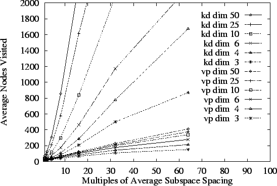
If this same database is now embedded into ever higher dimensions (3 through 50) and type 3 queries presented, Figure 8 results. In this graph, $\alpha$ (the amplitude of added noise) is expressed on the horizontal axis in normalized units.¹⁰The bottom group of six curves corresponds to vp-tree performance for range spaces of increasing dimension. The upper group provides kd-tree results. It is apparent that vp-tree performance degrades in a more reasonable fashion for queries increasingly distant from the data plane.

Figure 8: Off Data Plane Queries for Range Spaces of Increasing Dimension.

Similar results are obtained given much larger databases and given databases as simple as a mere line embedded in ${\mathbb{R}}^n$.

These results suggest that if one is given a database of unknown internal structure, the vp-tree may represent a better approach to organization for nearest neighbor retrieval.

Image Retrieval.

To test the method on a difficult real-world problem, a library of 16 B&W digital images measuring $604 \times 486$ pixels was built. Our metric space is the set of all fixed size subimages (windows). Sizes $4 \times 4$, $8 \times 8$, $16 \times 16$, $32 \times 32$, and, $50 \times 50$ are considered. So for example, a single library image corresponds to $260,715$ metric space elements of size $32 \times 32$.

The Euclidian metric is then applied and nearest neighbor retrieval effectiveness studied. The vp-trees built were very nearly balanced although large uniform regions (e.g. the sky) represent pathological subspaces creating occasional deep subtrees. Databases built from as many as 8 library images were considered corresponding to a metric space and vp-tree having over two million members.

For queries from the database, our depth-first branch and bound search reduces to standard binary tree search and the query is located without backtracking. Exactly $d$ node visits are then required where this refers to the depth in the tree of the element matching the query.

For queries even slightly distant from a database member, considerably more work is necessary. For window size $32 \times 32$ and trees of roughly one million elements, 5% of the nodes are visited on average to satisfy very near queries while 15% are visited in the general case.

In one series of experiments we choose subsets of four images each, and formed vp-trees. Searches were then performed using two query sources. The first source (general) consisted of a subset of six images different from each of the database images. The second source (similar) consisted of a pair of images captured so as to correspond very closely to a database image in each of the subsets. The results are summarized in table- 2 where the percentages shown are averages over the two databases.¹¹

Table 2: Image Search Results

Queries	$4\!\times\!4$	$8\!\times\!8$	$16\!\times\!16$	$32\!\times\!32$	$50\!\times\!50$
Similar	1.0%	3.4%	4.5%	4.5%	5.2%
General	1.4%	5.7%	10.7%	15.7%	19.3%

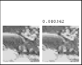
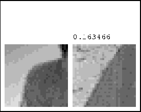
Figures 9 and 10 depict $32 \times 32$-pixel query/nearest-neighbor pairs for the similar and general cases respectively.¹²

Figure 9: A query (left) nearest neighbor pair where the query is drawn from an image very similar to one in the database.

Figure 10: A query (left) nearest neighbor pair where the query is drawn from an image entirely different from anything in the database.

Limited experiments with $\mbox{vp}^{\mbox{\footnotesize sb}}$-tree trees result in performance improvements that vary greatly, but seem to fall in the $15-30\%$ range.

We do not expect the kd-tree to perform well for large windows but perform experiments to verify our intuition. Indeed, little advantage is gained over exhaustive search for window sizes as small as $16 \times 16$.

Reducing search radius $\tau$ does decrease vp-tree search time but significant savings are achieved only at the expense of search effectiveness. In one experiment $\tau$ was reduced until search time was roughly halved. At this radius however, a nearest neighbor was located for only half of the queries. In another radius related experiment using single queries, we reduced $\tau$ to only slightly more than the known distance to their nearest neighbor - thus insuring search success. In one case, the nearest neighbor was located after only 1200 node visits, with an additional 13,799 required to complete the search. We offer this as illustration that finding a nearest neighbor and being sure are two separate matters - with the latter often dominating total cost.

This and other experiments suggest that heuristic search techniques represent an interesting area for further investigation. Indeed, independent of its ability to find nearest neighbors and prove it, the vp-tree method using only the simple search technique described, seems to very rapidly locate highly similar database elements. In some applications this may suffice.

Image searches with error tolerance (§3.4) also result in reduced work. Our limited experiments suggest however that reasonable tolerance values provide savings of at most perhaps a factor of two.

Finally, independent of search-time refinements, better data structures and construction techniques, represent a clear opportunity for future work.

Non-Euclidian Examples.

To illustrate the promised generality of our methods, two non-Euclidian cases are considered: 1) the pseudometric¹³that arises from normalized correlation. It measures the angle that two points form with the origin. and, 2) the ordinary Euclidian vector distance $d(X,Y)$ normalized by $(\Vert X\Vert+\Vert Y\Vert)$. That the result is a metric follows from a tedious argument provided in [27]. In both cases the vp-tree is applied to randomly constructed databases and exhibits search performance that corresponds well qualitatively to a standard Euclidian setting.

Concluding Remarks.

We have come to view the vp-tree construction and search processes as somewhat analogous to standard sort and binary search in one dimension - first because of their complexity, but perhaps more importantly because both primarily exploit ordinal rather than cardinal/representational information.

One may sort a file or build a binary tree of arbitrary objects given only an appropriate comparison function. By analogy, we have shown that a metric space may be organized for nearest neighbor retrieval given only the metric - without consideration of any particular representation such as a coordinate form. So for example, we will build the same vp-tree for a database in Euclidian space, independent of coordinate system.

We propose that techniques such as those of this paper should be used to develop application portable utility software for dynamic organization of and nearest neighbor retrieval from databases under application specific metrics.

Finally we observe that both kd-trees and vp-trees may be viewed as very special cases arising from particular uniformly continuous functionals and lying within the divide-and-conquer algorithmic paradigm. In one case coordinate projection, and in the other, distance from distinguished elements is used to hierarchically decompose space.

Acknowledgements.

I thank Eric Baum, Bill Gear, Igor Rivin, and Warren Smith for helpful discussions.

Bibliography

1

J. L. Kelly, General Topology.
New York: D. Van Nostrand, 1955.

2

B. V. Dasarathy, ed., Nearest neighbor pattern classification techniques.
IEEE Computer Society Press, 1991.

3

P. N. Yianilos, ``A dedicated comparator matches symbol strings fast and intelligently,'' Electronics Magazine, December 1983.

4

P. N. Yianilos, ``New methods for neighborhood searches in metric spaces.'' Invited Talk: The Institute for Defense Analyses, Princeton, NJ, July 23 1990.

5

J. K. Uhlmann, ``Satisfying general proximity/similarity queries with metric trees,'' Information Processing Letters, November 1991.

6

J. K. Uhlmann, ``Metric trees,'' Applied Mathematics Letters, vol. 4, no. 5, 1991.

7

W. A. Burkhard and R. M. Keller, ``Some approaches to best-match file searching,'' Communications of the ACM, vol. 16, April 1973.

8

K. Fukunaga, ``A branch and bound algorithm for computing k-nearest neighbors,'' IEEE Transactions on Computers, July 1975.

9

K. Fukunaga, Introduction to Statistical Pattern Recognition.
Academic Press, Inc., second ed., 1990.

10

G. Salton and A. Wong, ``Generation and search of clustered files,'' ACM Transactions on Database Systems, December 1978.

11

C. D. Feustel and L. G. Shapiro, ``The nearest neighbor problem in an abstract metric space,'' Pattern Recognition Letters, December 1982.

12

J. H. Friedman, F. Baskett, and L. J. Shustek, ``An algorithm for finding nearest neighbors,'' IEEE Transactions on Computers, October 1975.

13

J. H. Friedman, J. L. Bentley, and R. A. Finkel, ``An algorithm for finding best matches in logarithmic expected time,'' ACM Transactions on Mathematical Software, vol. 3, September 1977.

14

J. L. Bentley and J. H. Friedman, ``Data structures for range searching,'' Computing Surveys, December 1979.

15

J. L. Bentley, ``Multidimensional divide-and-conquer,'' Communications of the ACM, vol. 23, April 1980.

16

C. M. Eastman and S. F. Weiss, ``Tree structures for high dimensionality nearest neighbor searching,'' Information Systems, vol. 7, no. 2, 1982.

17

B. S. Kim and S. B. Park, ``A fast nearest neighbor finding algorithm based on the ordered partition,'' IEEE Transactions on Pattern Analysis and Machine Intelligence, vol. 8, November 1986.

18

A. J. Broder, ``Strategies for efficient incremental nearest neighbor search,'' Pattern Recognition, vol. 23, no. 1/2, 1990.

19

R. L. Rivest, ``On the optimality of Elias's algorithm for performing best-match searches,'' Information Processing 74, 1974.

20

T. P. Yunck, ``A technique to identify nearest neighbors,'' IEEE Transactions on Systems, Man, and Cybernetics, October 1976.

21

F. Aurenhammer, ``Voronoi diagrams - a survey of a fundemental geometric data structure,'' ACM Computing Surveys, vol. 23, September 1991.

22

P. M. Vaidya, ``An O(n log n) algorithm for the all-nearest-neighbor problem,'' Discrete & Computational Geometry, vol. 4, no. 2, pp. 101-115, 1989.

23

K. L. Clarkson, ``A randomized algorithm for closest-point queries,'' SIAM Journal on Computing, vol. 17, August 1988.

24

K. L. Clarkson, ``New applications of random sampling in computational geometry,'' Discrete & Computational Geometry, vol. 2, pp. 195-222, 1987.

25

A. M. Frieze, G. L. Miller, and S.-H. Teng, ``Separator based parallel divide and conquer in computational geometry,'' SPAA 92, 1992.

26

D. Dobkin and R. J. Lipton, ``Multidimensional searching problems,'' SIAM Journal on Computing, vol. 5, June 1976.

27

P. N. Yianilos, ``Normalized forms for two common metrics,'' tech. rep., The NEC Research Institute, Princeton, New Jersey, December 1991.

About this document ...

Data Structures and Algorithms for Nearest Neighbor Search in General Metric Spaces

This document was generated using the LaTeX2HTML translator Version 2K.1beta (1.47)

Copyright © 1993, 1994, 1995, 1996, Nikos Drakos, Computer Based Learning Unit, University of Leeds.
Copyright © 1997, 1998, 1999, Ross Moore, Mathematics Department, Macquarie University, Sydney.

The command line arguments were:
latex2html -split 0 -image_type gif -nonext_page_in_navigation -noprevious_page_in_navigation -up_url ../main.html -up_title 'Publication homepage' -numbered_footnotes vptree.tex

The translation was initiated by Peter N. Yianilos on 2002-07-07

Footnotes

... 1986-87¹

First coded and tested in July of 1987 during a Proximity Technology Inc. company workshop in Sunnyvale California. Participants in addition to the author were Samuel Buss (then at U.C. Berkeley/Mathematics), Mark Todorovich, and Mark Heising.

... relation²

Bounded metrics may simply be scaled. Unbounded metrics may be adjusted using the well known formula: $\bar{d}(a,b) = \frac{d(a,b)}{1+d(a,b)}$.

... generality³

The method of compression may affect search efficiency/time, but not the result.

... drawn⁴

We can do this in general by choosing the smallest sigma-algebra containing the space's metric topology, and defining a measure on it.

... returned.''⁵

... tree⁷

And we've not considered the issue of median ambiguity.

... vp-tree⁸

In all of our experiments, fixed sample sizes are employed to choose and evaluate vantage points. In hypercube settings, we evaluate $100$ random vantage point candidates by computing their distance to $100$ random database elements. For image experiments, only $10$ candidates are drawn.

... node⁹

There are 4,000 total.

... units.¹⁰

The unit consists of the average distance from a type 1 query to its nearest neighbor. So $\alpha=1$ then corresponds to added ${\mathbb R}^n$ noise of comparable amplitude.

... databases.¹¹

Our use of a pair of databases represents a crude statistical precaution necessary due to the small number of images we can computationally afford to deal with. Despite this measure, and our careful attempts to build a varied image set, we are mindful of the fact that the entire space of naturally occurring images is immense indeed in comparison with our experiments. One should therefore not conclude that the statistics we report are representative of the fully general case.

... respectively.¹²

The value displayed in these figures represents Euclidian distance between the query/database-element pair.

... pseudometric¹³

Our methods have been presented for metric spaces only but may be generalized to pseudo-metric spaces.