Excluded Middle Vantage Point Forests for Nearest Neighbor Search

Peter N. Yianilos¹

July 20, 1998

Abstract:

The excluded middle vantage point forest is a new data structure that supports worst case sublinear time searches in a metric space for nearest neighbors within a fixed radius $\tau$ of arbitrary queries. Worst case performance depends on the dataset but is not affected by the distribution of queries.

Our analysis predicts vp-forest performance in simple settings such as $L_p$ spaces with uniform random datasets -- and experiments confirm these predictions. Another contribution of the analysis is a new perspective on the curse of dimensionality in the context of our methods and kd-trees as well. In our idealized setting the dataset is organized into a forest of $O(N^{1-\rho})$ trees, each of depth $O(\log{N})$. Here $\rho$ may be viewed as depending on $\tau$, the distance function, and on the dataset. The radius of interest $\tau$ is an input to the organization process and the result is a linear space data structure specialized to answer queries within this distance. Searches then require $O(N^{1-\rho} \log{N})$ time, or $O(\log{N})$ time given $O(N^{1-\rho})$ processors.

Our conclusion is that these new data structures exhibit useful behavior only for small radius searches, where despite their variation in search times, conventional kd-trees perform much better.

Keywords: Nearest neighbor search, Vantage point tree (vp-tree), kd-tree, Computational geometry, Metric space.

Introduction

We consider the radius-limited nearest neighbor problem in a metric space. That is, given an $N$ point dataset and a radius of interest $\tau$, produce a data structure and associated search algorithm to rapidly locate the dataset point nearest to any query $q$. Our focus is on practical data structures that provide worst-case search time bounds.

Vantage point trees (vp-trees) [32] and kd-trees [15,16,4,3] organize an $N$ point dataset so that sublinear time nearest neighbor searches may be performed on an expected basis for some fixed distribution. Performance depends on the dataset and on the assumed distribution of queries.

The excluded middle vantage point forest (vp-forest) is a new related data structure that supports worst case sublinear time searches for nearest neighbors within a fixed radius $\tau$ of arbitrary queries. Worst case performance depends on the dataset but is not affected by the distribution of queries.

The dataset is organized into a forest of $O(N^{1-\rho})$ trees, each of depth $O(\log{N})$. Here $\rho$ may be viewed as depending on $\tau$, the distance measure, and on the dataset. The radius of interest $\tau$ is an input to the organization process and the result is a data structure specialized to answer queries within this distance.

Each element of the dataset occurs in exactly one tree so that the entire forest remains linear space. Searches follow a single root-leaf path in each tree. There is no backtracking when the search is limited to neighbors within distance $\tau$. Along its way every neighbor within $\tau$ is necessarily encountered. The query's effect is to guide the descent through each tree.

There are no significant ancillary computational burdens at search time. So upon creating the forest, the user simply adds the depths of each tree in the forest to arrive at the maximum number of distance evaluations each search will require. Each tree may be searched independently. Searches then require $O(\log{N})$ time given one processor for each tree in the forest.

We also discuss design variations that trade space for reductions in search time -- and compare forests with single trees constructed similarly.

The general idea behind vp-forests is easily understood. Both vp-trees and kd-trees recursively divide the dataset. At each node the remaining dataset elements have an associated value, and the node has a corresponding fixed threshold that is roughly central in the distribution of values. Elements below this threshold are assigned to, say, the left child, and those above to the right. For kd-trees these values are those of individual coordinates within each data vector. For vp-trees they are the distance of a metric space element to some fixed vantage point.

Elements near to the threshold lead to backtracking during search. When building a vp-forest, such elements are deleted from the tree and added instead to a bucket. Once the tree is complete, the bucket is organized into a tree in the same way, resulting in another (smaller) bucket of elements. This continues until the forest is built. This effectively eliminates backtracking. Because elements near to the threshold are recursively deleted, and this threshold lies near the middle of the distribution of values, we refer to our data structure as an excluded middle vantage point forest. Both vp-trees and kd-trees may be regarded as trivial instances of vp-forests with no excluded middle.

We present an idealized analysis that allows us to predict vp-forest performance in simple settings such as $L_p$ spaces with uniform random datasets. Experiments are reported that confirm these predictions. One contribution of this analysis is an interesting new perspective on the so called curse of dimensionality (that is that nearest neighbor search increases in difficulty with dimension). In Euclidean space given a uniform random dataset drawn from the hypercube, we observe that the worst-case difficulty of vp-forest search for any fixed $\tau$ ought to be asymptotically constant with respect to dimension -- and our experiments confirm this. Using $L_1$ we expect constant difficulty if $\tau$ is allowed to increase with $d^{1/2}$ ($d$ denotes dimension), and this too is confirmed by experiment.

Our analysis also suggests that kd-trees should exhibit the same dimension invariance for fixed search radii, and experiments confirm this. For a worst case query, kd-tree search visits essentially the entire dataset, but on average performs far less work than the vp-forest.

The vp-forests described in this report stimulated the developments of [33], but do not themselves appear to have immediate practical value.

We conclude our introduction with a brief discussion of the nearest neighbor search problem and literature. See [32] for additional discussion.

Nearest neighbor search is an important task for non-parametric density estimation, pattern recognition, information retrieval, memory-based reasoning, and vector quantization. See [11] for a survey.

The notion of a mathematical metric space [20] provides a useful abstraction for nearness. Examples of metric spaces include Euclidean space, the Minkowski $L_p$ spaces, and many others. Exploiting the metric space triangle inequality to eliminate points during nearest neighbor search has a long history. Our work belongs to this line. This paper extends it by i) introducing structures that give worst case time bounds for limited radius searches, ii) providing analysis for them, iii) introducing a method for trading space for time, and iv) defining our data structures and algorithms in terms of abstract projectors, which combines approaches that use distance from a distinguished element with those such as kd-trees that use the value of a distinguished coordinate.

In early work Burkhard and Keller [7] describe methods for nearest neighbor retrieval by evaluating distances from distinguished elements. Their data structures are multi-way trees corresponding to integral valued metrics.

Fukunaga in [18,19] exploits clustering techniques [27] to produce a hierarchical decomposition of Euclidean Space. During a branch and bound search, the triangle inequality is used to rule out an entire cluster if the query is far enough outside of it. While exploring a cluster he observes that the triangle inequality may be used to eliminate some distance computations. A key point missed is that when the query is well inside of a cluster, the exterior need not be searched.

Collections of graphs are considered in [14] as an abstract metric space with a metric assuming discrete values only. This work is related to the constructions of [7]. In their concluding remarks the authors clearly anticipate generalization to continuous settings such as ${\mathbb{R}}^n$.

The idea that vantage points near the corners of the space are better than those near the center was described in [28] and much later in [32].

More recent papers describing vantage-point approaches are [30,29,25] and [32] who describe variants of what we refer to as a vantage-point tree. Also see [10] for very recent work on search in metric spaces.

The well-known kd-tree of Friedman and Bentley [15,16,4,3] recursively divides a pointset in ${\mathbb{R}}^d$ by projecting each element onto a distinguished coordinates. Improvements, distribution adaptation, and incremental searches, are described in [13], [21], and [6] respectively. In our framework kd-trees correspond to unit vector projection with the canonical basis.

More recently, the Voronoi digram [2] has provided a useful tool in low- dimensional Euclidean settings - and the overall field and outlook of Computational Geometry has yielded many interesting results such as those of [31,9,8,17] and earlier [12]. It appears that [12] may be the first work focusing on worst case bounds.

Very recently Kleinberg [22] gives two algorithms for an approximate form of the nearest neighbor problem. The space requirements of the first are prohibitive but the second, which almost always finds approximate nearest neighbors seems to to be of more practical interest. The recent work reported in [1] also considers an approximate form of the problem. Their analysis gives exponential dependence on $d$ but the heuristic version of their approach they describe may be of practical interest.

For completeness, early work dealing with two special cases should be mentioned. Retrieval of similar binary keys is considered by Rivest in [26] and the $L_\infty$ setting is the focus of [34].

See [5] for worst case data structures for the range search problem. This problem is related to but distinct from nearest neighbor search since a neighbor can be nearby even if a single coordinate is distant. But the $L_\infty$ nearest neighbor problem may be viewed as an instance of range search. Their paper also describes a particular approach to trading space for time via an overlapping cover. Our discussion of this topic in section 5 also takes this general approach.

Vantage Point Forests

We begin by formalizing the ideas and construction sketched in the introduction.

Definition 1   Consider an ordered set $X = \{x_1,\ldots,x_N\}$ and a value $m \in [0,1]$. Let $w = \lfloor mN \rfloor$ and $a = \lfloor (N-w)/2 \rfloor$. Then the $m$-split of $X$ consists of left, middle, and right subsets defined by:

$$\begin{eqnarray*} L & = & \{x_i \vert i \leq a \} \\ M & = & \{x_i \vert i > a, i \leq a+w \} \\ R & = & \{x_i \vert i > a+w \} \end{eqnarray*}$$

That is, a balanced 3-way partition of $X$ with a central proportion of approximately $m$.

Algorithm 1   Given a collection of points $H$ and a 1-1 projection function $\pi_G: H \rightarrow {\mathbb{R}}$ defined for any nonempty $G \subseteq H$, define $\pi_G(G)$ to be the ordered set of distinct real values corresponding to the image of $G$ under $\pi_G$. Now for $m \in [0,1]$:

1. consider the $m$-split $L,M,R$ of $\pi(G)$, and define the split $G_L, G_M, G_R$ of $G$ corresponding to the preimages of $L,M,R$ respectively.

2. Given $G \subseteq H$ construct a binary tree by forming $G_L, G_M, G_R$, discarding $G_M$, and then doing the same recursively for $G_L$ and $G_R$ until single elements remain forming the tree's leaves.

3. Starting with $H$ build a tree $T_1$ as described above and denote its membership by $M_1$. Let $H_0 = H$ and define $H_1 = H_0 - M_1$, i.e. the elements discarded building $T_1$.

4. For $k > 1$ and $H_{k-1} \neq \emptyset$ define $T_k$ as the tree built as above for $H_{k-1}$, denote the tree's membership by $M_k$, and define $H_k = H_{k-1} - M_k$.

Definition 2   We refer to the result of algorithm 1 as the idealized excluded middle vantage point forest induced by $\pi$ with central proportion $m$. When $H$ is a metric space and the projection functions $\pi$ satisfy $\vert \pi(x) - \pi(y) \vert \leq d(x,y), \forall x,y \in H$, this forest is of use for nearest neighbor search and we further define $\tau$ to be one half of the minimum diameter of a middle set discarded during construction.

We remark that each tree of the forest may be viewed as analogous to the Cantor set from real analysis. That is, the subset of $[0,1]$ constructed by removing the central third of the interval -- and proceeding recursively for both the left and right thirds. Our forest then corresponds to a decomposition of the space into a union of Cantor sets.

Two important examples of a suitable family of $\pi$ functions are vantage point projection for general metric spaces, and unit vector projection for Euclidean space.

A vantage point projector $\pi_p$ is defined for any $p \in H$ by $\pi_p(x) = d(p,x)$. The split points in tree construction correspond to abstract spheres about $p$. It is easily verified that $\vert \pi_p(x) - \pi_p(y) \vert \leq d(x,y)$ as required. The range of this projector is the nonnegative reals. Letting $m=0$ gives rise to a vantage point tree [32].

The unit vector projector $\pi_p$ is defined for any $p \neq 0$ as $\pi_p(x) = <p,x>/\Vert p\Vert$. This is easily seen to satisfy the required inequality as well, and its range is not limited to nonnegative values. Here the split points correspond to hyperplanes. Choosing $p$ as canonical unit vectors and letting $m=0$ builds a form of kd-tree [15,16,4,3]. It is important to note that $<p,x>$ may be computed more rapidly for canonical unit vectors -- in constant time with respect to dimension. Also, we remark that whenever orthogonal vectors are used, projection distances are, in a sense, additive, and that this fact can be exploited (as kd-trees do) when designing solutions specialized for $L_p$ spaces. We do not consider either of these optimizations in this paper.

Proposition 1   Consider an idealized Vantage Point Forest with central proportion $m$ and corresponding value $\tau$. Define $\rho = 1/(1-\log_2{(1-m)})$. Then:

1. There are $\Theta(N^{1-\rho})$ trees in the forest, having maximum depth $\Theta(\log{N})$.

2. A search for nearest neighbors within distance $\tau$ of a query requires $\Theta(N^{1-\rho} \log{N})$ time, and linear space -- independent of the query.

3. The search requires $\Theta(\log{N})$ time given $\Theta(N^{1-\rho})$ independent processors.

4. Assuming each projector $\pi_G$ can be constructed in constant time, and that it can also be evaluated in constant time, and that $m > 0$, then $O(N^{2-\rho})$ time is required to construct the forest.

proof: At each step in the construction the central proportion of $m$ elements is removed so that the left and right subsets are each of size $(1-m)/2$. The first tree's depth is then $[1/log_2(2/(1-m))] log_2 N = \Theta(\log N)$. So the number of elements left in the tree is $N^{1/(1-log_2(1-m))} = N^\rho$.

The number of elements left after the first tree has been constructed is then $N - N^\rho$. After the second $N - N^\rho - (N - N^\rho)^\rho$ are left, and so on. Clearly $\Omega(N^{1-\rho})$ trees are required to reduce the population to any fixed size.

Once the population has been reduced to $1/2$ of its original size, the number of elements removed as each tree is built will have declined to $(N/2)^\rho = (1/2)^\rho N^\rho$. Since $(1/2)^\rho > 1/2$ no fewer than $N^\rho / 2$ are removed. So the number of steps required to reach $N/2$ is no more than $N^{1-\rho}$. The number required to reach $N/4$ is then $(1/2)^{1-\rho} N^{1-\rho}$ -- and so on forming a geometric series. So the number required to reach any fixed level is $O(N^{1-\rho})$. The number of trees in the forest is then $\Theta(N^{1-\rho})$ -- and the total space is clearly linear.

A search for nearest neighbors within distance $\tau$ is then made by following a single root-leaf path in each tree establishing the required time bound. Each tree can be considered independently and the results merged to arrive at a single nearest neighbor. This establishes the stated parallel complexity.

Finally we consider organizational time. The first level of the first tree requires $O(N)$ work to produce projection values of each point in the space, and then $O(N)$ time to effect the split (linear time order statistics). The next level considers a total of $(1-m)N$ records, and so on, leading to $O(N)$ overall time from which the stated organization time bound follows.$\;\Box$

For example, if $m=1/2$ there are $O(\sqrt{N})$ trees in the forest, and search time is $O(\sqrt{N} \log{N})$. Organization requires $O(N^{3/2})$ time, but as always only $O(N)$ space is consumed. As $m \rightarrow 1$ we expect $\tau$ to increase but the number of trees approaches $N$ and searches come ever closer to examining every point. As $m \rightarrow 0$ we expect $\tau$ to decrease while search time approaches the logarithmic ideal. The $m$ parameter then, in a sense, interpolates between exhaustive large-$\tau$ search, and logarithmic small-$\tau$ search.

Our development above is very general and describes idealized forests. We now explain in what sense they are idealized and begin our discussion of concrete settings.

Algorithm 1 removes a fixed central proportion of the points as each tree node is processed. This simplifies analysis but, because $\tau$ is defined as the minimum diameter of all such central cuts, $\tau$ might wind up too small to be of any practical value. Also, the projection function will not in general be 1-1, and this detail must be considered in any implementation. The user's objective is a satisfactory tradeoff between the conflicting goals of minimizing search time, and maximizing $\tau$.

One approach is to minimize search time given a lower bound on $\tau$. In contrast with the idealized case, here it makes sense to cut a variable central proportion -- one of diameter $2 \tau$. Notice in this case that the construction recursion may terminate before reaching a single node. Since the choice of projector may affect this proportion, it may be wise to invest additional time during construction to evaluate multiple projectors. This corresponds to the idea of selecting a vantage point for a vp-tree, or a cut-dimension for a kd-tree. When fixed diameter cuts are made a more complicated stopping rule for forest construction is needed. Otherwise a tiny ball of points, smaller than $2 \tau$ in diameter, will never be assigned to any tree.

It is also important to note that while our focus is on worst case performance, and there is no backtracking required to search for neighbors within distance $\tau$, that backtracking can be performed as for vp-trees or kd-trees in order to satisfy queries beyond $\tau$.

Another difference between our idealized construction and practical implementations is that in the idealized case points are stored only at tree leaves.

In the vp-tree case the projector is formed by selecting an element $v$ of subspace $G$ and computing its distance to the query $q$ and to every other element of $G$. Having computed its distance to the query, there is no need to examine $v$ again, and we therefore view it as stored at the interior tree node at which is was used. So the difference is that the set $G - \{v- \}$ is split at each level of the recursion. When using unit vector projection it is also possible to use an element $x$ of the database. Here too, it is unnecessary to examine $x$ again since $d(x,q)$ is easily computed given $<x,q>$.

Performance in $L_p$ spaces

The Minkowski $p$-norm is denoted $L_p$ and defined by $\Vert X\Vert _p = (\sum_i \vert x_i\vert^p)^{1/p}$ for $p \geq 1$. A metric results from evaluating the norm of the difference of two vectors. The Euclidean metric is $L_2$, the city block metric is $L_1$, and by convention $L_\infty$ gives the maximum absolute value over individual coordinates.

We begin with an asymptotic statement that allows to understand the expected performance of excluded middle vantage point forests in high dimensional instances of these spaces given distributions such as the uniform one.

Proposition 2   Let $X \triangleq (x_1,\ldots,x_d)$ be a vector of i.i.d. random variables. Consider $Y \triangleq \Vert X\Vert _p$ and let $\sigma^2$ denote the variance of $Y$ about its mean. Then $\sigma = \Theta(d^{1/p - 1/2})$ regarding $p$ is fixed and letting $d \rightarrow \infty$.

proof: Consider $Y^p = \sum_{i=1}^d \Vert x_i\Vert^p$. Because the $x_i$ are i.i.d. both the mean and variance of $Y^p$ scale linearly with $d$. So relative to the magnitude of the mean of $Y^p$, its standard deviation shrinks as $d^{-1/2}$, whence the distribution of $Y^p$ values is increasingly concentrated about its mean. Taking the $p$th root to arrive at $Y$ has the effect of scaling all of these values downward by a factor of approximately $d^{1/p}/d = d^{(1/p) - 1}$ so the variance changes by a factor of $d^{(2/p)-2}$. But the variance of $Y^p$ scales with $d$, so the variance of $Y$ scales with $d^{(2/p)-1}$, and its standard deviation with $d^{1/p - 1/2}$.$\;\Box$

To keep its statement simple the proposition includes an i.i.d. assumption, but less is necessary. Independence is required but the mean and variance of each variable $x_i$ need not be the same. It is merely necessary that the mean and variance of $Y^p$ scales approximately linearly with $d$.

The proposition is then relevant because of two observations about uniformly distributed high dimensional $L_p$ spaces. Firstly, that choosing a point $v$ at random, the distribution of $\Vert x-v\Vert _p^p$ over $x$ in the space exhibits the required linear scaling behavior. Secondly, that making cuts during construction (whether spherical or hyperplanar) in a high dimensional space, leaves subspaces that for the purposes of this proposition still behave like uniformly random ones. The same is true for unit vector projection.

For Euclidean space ($p=2$) we then expect $\sigma$ to be asymptotically constant with dimension. Then the distribution of values the construction algorithm is presented with at each step, becomes the same for sufficiently high dimension. For $L_1$ we have that $\sigma$ scales upward with $d^{1/2}$, and for $L_\infty$ it scales downward with $d^{-1/2}$. The result is that we expect the following behavior when using excluded middle vantage point forests to search uniformly distributed point sets:

1. The worst-case time to search for the nearest neighbor within distance $\tau$ of a query under the Euclidean metric, is constant with respect to dimension.

2. Using $L_1$ the task becomes easier with increasing dimension, or, one can scale $\tau$ upward with $d^{1/2}$ and maintain constant time.

3. For $L_p, p > 2$ the task becomes harder with increasing dimension. Interestingly, in the limiting $L_\infty$ case, our approach is essentially worthless but range search techniques apply because a search for neighbors within $\tau$ is just a range query of this form applying to every dimension.

Finally we remark that the case of unit vector projection in Euclidean space directly leads to the first observation above without the proposition.

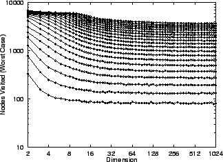
We have implemented our ideas as an ANSI-C program. Figures 1 and 2 describe experiments which confirm the behavior above for $L_1$ and $L_2$. It is important to reiterate that searching the forest involves no decisions or backtracking, so that search time is essentially constant. So:

1. Our experiments reflect the time required to perform the search for any given query.

2. Because of the nature of the search, all neighbors within $\tau$ will necessarily be encountered during it.

Other experiments confirmed the expected behavior when $p > 2$. Vantage point projection is used but unit vector projection gives similar results. A vantage point is selected at random from the current subset of the dataset. The implementation forces fixed $\tau$ cuts and stops forest construction when all remaining points are failed to be assigned to a tree after a large number of attempts. These points are then stored as a simple list. The implementation also stores points at interior nodes, not just at leaves. Finally, its splitting algorithm is general, i.e. does not assume 1-1 projection functions.

Figure 1: The worst-case number of nodes visited by an excluded middle vantage point forest search under the $L_2$ metric $(p=2)$, the uniform distribution (10,000 points), and fixed $\tau$ radius, does not in the limit depend on dimension. The curves depicted from bottom to top correspond to central exclusion widths from $0.05$ to $1.00$ in increments of $0.05$. Corresponding $\tau$ values are half as large.

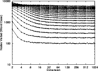Figure 2: For the $L_1$ metric $(p=1)$ and the setting of figure 1, dimension invariance is observed if central exclusion widths are scaled by $\sqrt {d}$. For example, the bottom curve corresponds to $\tau = 0.025$ for $d=2$ and $\tau = \sqrt {512/2} \times 0.025 = 0.4$ for $d = 512$. So for $L_1$ the search radius may increase with dimension while holding worst-case performance constant.

The uniform random case is, of course, of little practical interest. While we give no general worst case bounds it is important to note that performing a fixed $\tau$ construction will always generate a forest, and a corresponding query-independent worst case bound on search time for that particular point set.

We compare performance in our setting with kd-tree search [15,16,4,3], adapted from [23] as described in [33] for radius limited search.

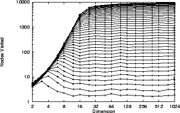
Figure 3 shows the result of our experiment. The same dimensional invariance is evident, but now with respect to expected search time. As for our worst-case structures, this follows from our earlier observations about projection distributions in high dimensional spaces. The figure shows that expected search complexity is somewhat lower than the worst case results of figure 1 where saturation is evident exclusion width $1$ is approached. For kd-trees, saturation is delayed until roughly width $2$.

The expected kd-tree search times are much lower than the worst case values of figure 1. In fact, given random queries, the probability is vanishingly small that kd-tree search will cost as much as our worst case search.

In the uniform case a query at the center of the hypercube is costly for the kd-tree, and we have confirmed that essentially the entire dataset is searched in this case. We observe that one might build a pair of kd-trees whose cut points are offset to eliminate these hot spots and perhaps even provide worst case performance bounds in the radius-limited case.

Figure 3: The average number of nodes visited by kd-tree search under the $L_2$ metric $(p=2)$, the uniform distribution (10,000 points), and fixed $\tau$ radius, does not in the limit depend on dimension. The curves depicted from bottom to top correspond to central exclusion widths from $0.05$ to $2.00$ in increments of $0.05$. Corresponding $\tau$ values are half as large.

Excluded middle trees vs. Forests

By slightly modifying the forest construction algorithm one can build a single 3-way tree. Instead of adding the central elements to a bucket for later use in building the next tree, we instead leave them in place forming a third central branch. To search such a tree one must follow two of the three branches: either the left and middle, or the middle and right. We remark that this tree structure was our first idea for enhancing vantage point trees to provide worst-case search time bounds.

Like the forest, this tree requires linear space, but a simple example and analysis illustrates that its search performance is usually much worse.

Consider the 3-way tree built by an equal 3-way division, i.e. where the central exclusion proportion is $1/3$. Then the tree's depth is $\log_3{N}$. The path taken by any single search consists of a binary tree embedded within this trinary tree. So $N^{\log_3 2} \approx N^{0.63}$ nodes will be visited. But we have seen that a forest with exclusion proportion $1/2$ results in $O(N^{0.5} \log{N})$ node visits, which is superior despite the fact that the tree was built using a smaller exclusion proportion ($1/3$ vs. $1/2$).

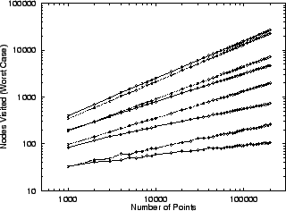
Table 4 compares the performance of idealized trees and forests for various database sizes and central exclusion proportions. Figure 4 compares the performance of actual trees and forests in a uniform distribution Euclidean space setting. The results are consistent with our analysis and the computations of table 4. We briefly remark that for small $\tau$, trees and forests with a higher branching factor make sense. Here the projected point set is partitioned into bands with alternating ones corresponding to the excluded middle of our 3-way construction.

Table 1: The relative search time ratio of an idealized excluded middle vantage point forest, to that of a tree. The forest is better in almost all cases. Notice that its relative advantage can be quite large. The tree is preferred only in the case of large central exclusion widths, and then by only a small factor.

Central	Number of Elements
Proportion	$10^{3}$	$10^{4}$	$10^{5}$	$10^{6}$	$10^{7}$	$10^{8}$
0.100	0.52	0.37	0.23	0.14	0.08	0.05
0.300	0.87	0.58	0.42	0.29	0.18	0.11
0.500	1.21	0.96	0.83	0.63	0.44	0.36
0.700	1.40	1.31	1.18	1.03	0.88	0.77
0.900	1.50	1.64	1.65	1.58	1.51	1.51

Figure 4: A comparison of excluded-middle vantage trees (dashed line) and forests (solid line) for the $L_2$ metric, $d=64$, the uniform distribution, and central exclusion widths of $0.01, 0.10, 0.25$, and $0.50$ corresponding to the curve pairs from bottom to top. For small widths the forest performs better and the advantage increases with database size (see the difference in curve slopes). This advantage reduces with increasing exclusion width, and by $0.50$ the tree is the winner.

Trading Space for Time

Until now we have considered linear space structures. In this section we describe a general technique for trading space for time. For analysis we will return to the idealized setting in which construction removes fixed proportions -- not fixed diameter central subsets as in the implementation and experiments. This will allow us to make calculations intended to illuminate the engineering tradeoffs one faces in practice.

The 3-way split performed by algorithm 1 is illustrated in figure 5(a). The central proportion $m$ is imagined to correspond to some fixed radius $\tau$ as shown. We motivate the construction in terms of $\tau$ but will analyze it in terms of $m$.

Figure 5: a) An idealized illustration of the division according to definition 1 of the projection of a point set onto the real line. Subset $M$ results from removing the central proportion of $m$ elements. Assuming a symmetrical distribution set $M$ has diameter $2 \tau$. Subset $L$ consists of everything below $M$ in projected value, and $R$ of everything above it. b) An idealized illustration of the tradeoff of space for time. Here an additional proportion $m_x$ of central elements encloses $M$ and corresponds to two subsets $R_x$ and $L_x$. Elements of $R_x$ are stored in $R$ and also in $L$. Likewise elements of $L_x$ are stored in both $L$ and $R$. The result is that the effective search radius within which the worst case time bound holds is extended from $\tau$ to $\tau +\tau _x$.

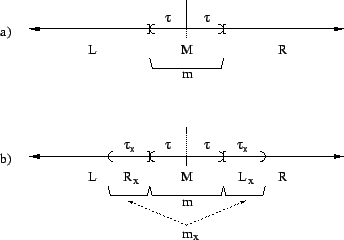When the projection of a query lies just to the right of the dotted centerline, a search for a nearest neighbor within $\tau$ will explore $M$ and $R$. Increasing $\tau$ by some value $\tau_x$ forces the search to explore $L$ as well.

To avoid exploring all three we store the points in interval $R_x$ in two places (see figure 5(b)). First, they are stored as always in $L$. Second, they are stored with those of $R$. As a result of this overlap only $M$ and $R$ must be explored as before. Points in interval $L_x$ are similarly stored twice.

Continuing this modified division throughout forest construction yields a data structure that:

1. Includes the same number of trees as before, since the size of the excluded central proportion is unchanged.

2. Contains trees that are deeper, but still asymptotically of logarithmic depth. Tree depth is $\log_{\frac{2}{(1-m+m_x)}} N$.

3. The result is the same worst-case asymptotic search times, but over the larger idealized radius $\tau +\tau _x$.

4. Provides this search-time benefit at the cost of space. The deeper tree has $N^{\frac{1}{\log_2{\frac{2}{(1-m+m_x)}}}}$ nodes. Space for the entire forest is then:

   
   

   $$O(N^{1 + \frac{1}{\log_2{\frac{2}{1-m+m_x}}} - \frac{1}{1 - \log_2{1-m}}})$$
   
   

For example, let $m=1/2$ and $m_x = 1/4$. Then space is $\approx O(N^{1.2067})$.

From another viewpoint the same space tradeoff may be used to reduce search time for a fixed $\tau$. For example, an ordinary $m=0.5$ forest provides $O(N^{0.5} \log{N})$ searches. Letting $m=0.25$ and $m_x = 0.25$ reduces the time to $\approx O(N^{0.2933} \log N)$ but space is increased from $O(N)$ to $\approx O(N^{1.2933})$.

Finally consider the interesting extreme case where $m=0$. Here the forest consists of a single binary tree. Search time is then $O(\log{N})$ with space $O(N^{\frac{1}{\log_2{\frac{2}{1+m_x}}}})$.

Some Topics for Future Work

Excluded middle forests might be applied to problems other than nearest neighbor search. They might, for example, improve the effectiveness of decision trees, an important tool for machine learning [24]. The motivation here is that values near to the decision threshold may be more difficult to classify based on the selected decision variable.

We now discuss several possibilities related to nearest neighbor search. For each fixed $\tau$ our implementation generates a forest with some associated worst case query time bound. Smaller $\tau$ values, in general, result in smaller bounds. Now suppose that a forest is built with $\tau=1$ and the system is then presented with a query. Next suppose that early in the search a neighbor is encountered that is well within the $\tau$ radius, say at distance $0.3 \tau$. Despite our good fortune the remaining search will take no less time. Root-leave paths in every remaining tree must be examined.

One idea is to build multiple forests. One for $\tau=1$, and additional forests for $\tau=1/2, 1/4, 1/8$, etc. Then upon encountering a point at distance $0.3 \tau$ the search algorithm might consider aborting its processing of the $\tau=1$ forest and switch over to the $\tau=1/2$ forest, which offers a better worst case time bound.

It is interesting to note that this decision to switch can be made very easily by considering the number of points remaining in the current forest, and comparing it to the worst case bound for the new one. If the latter is smaller it makes sense to switch over. Implementations may consider another factor in their decisions. The distance from the query to all points already visited might be remembered to avoid unnecessary metric evaluations when processing restarts at the beginning of a new forest.

Another topic for future work involves two settings in which our methods seem far from optimal: boolean vectors with Hamming distance, and the $L_\infty$ case.

The boolean Hamming distance setting corresponds to $L_1$, and the number of errors we can tolerate while maintaining constant search complexity for the uniform distribution grows with $d^{1/2}$. But experiments suggest that our forests do not compete in practice with a particular simple method. If $\tau$ is the maximum Hamming distance to be tolerated, this method divides the high-dimensional vector into $\tau+1$ segments and exploits the fact that the dataset projected onto one of these segments may be assumed to have Hamming distance zero to the query. Simple hashing may then be used to maintain these projections. We are interested in better understanding the relationship of this simple technique to the ideas of this paper. We remark that the same idea of dimensional partitioning applies to any Minkowski metric, but so far we can obtain an advantage only in the Boolean case.

As described earlier, our methods grow weaker with growing $p$, becoming essentially useless for $L_\infty$. This is interesting since suddenly, with $p=\infty$, the problem becomes an instance of range search. We speculate that ideas from range search might in some form be of use before $p$ reaches $\infty$ -- if only as an approximate solution to the nearest neighbor problem.

Finally we observe that in ${\mathbb{R}}^d$ storing the data vectors themselves requires $O(n d)$ space. The tree/forest we build can use $O(1)$ space pointers to these vectors. For this reason we can tolerate super-linear space in the tree/forest, namely $O(n d)$. We suggest that a practical implementation for Euclidean space should take advantage of this and also exploit the canonical/orthogonal basis optimizations mentioned in section 2.

Towards a General High-Level Procedure for Nearest Neighbor Search

Our work towards a general and practical tool for nearest neighbor search began with [32] and continues with this paper. We envision a high-level procedure that like the qsort() function from the standard Unix library, views its underlying database through a layer of abstraction. In the case of sorting, a comparison function is provided. For nearest neighbor search projection and distance computation must be supported.

Sorting is, however, a much simpler problem in as much as practical algorithms exist with acceptable worst case time and space complexity -- independent of the dataset. For nearest neighbor search we suggest that a general tool must be flexible and support:

• User supplied metrics and projectors.
• The construction of dataset-specific solutions giving worst-case query times for neighbors within a specified distance.
• Heuristic backtracking searches beyond this distance.
• Control over the time invested in construction to optimize the resulting data structure.
• Control over the time-space tradeoff. That is, the ability to invest additional space to improve search performance.
• Dynamic operation, i.e. the addition and deletion of points from the data structure during use (not discussed in this paper -- but clearly possible).
• The ability to exploit the canonical/orthogonal basis optimizations for $L_p$ mentioned in section 2.

We hope that the ideas and results of this paper brings us closer to the development of such a tool.

Acknowledgements

The author thanks Joe Kilian for helpful discussions.

Bibliography

1

ARYA, S., MOUNT, D., NETANYAHU, N., SILVERMAN, R., AND WU, A.
An optimal algorithm for approximate nearest neighbor searching in fixed dimension.
In Proc. 5th ACM-SIAM SODA (1994), pp. 573-583.

2

AURENHAMMER, F.
Voronoi diagrams - a survey of a fundemental geometric data structure.
ACM Computing Surveys 23, 3 (September 1991).

3

BENTLEY, J. L.
Multidimensional divide-and-conquer.
Communications of the ACM 23, 4 (April 1980).

4

BENTLEY, J. L., AND FRIEDMAN, J. H.
Data structures for range searching.
Computing Surveys (December 1979).

5

BENTLEY, J. L., AND MAURER, H. A.
Efficient worstcase data structures for range searching.
Acta Informatica 13, 2 (1980), 155-168.

6

BRODER, A. J.
Strategies for efficient incremental nearest neighbor search.
Pattern Recognition 23, 1/2 (1990).

7

BURKHARD, W. A., AND KELLER, R. M.
Some approaches to best-match file searching.
Communications of the ACM 16, 4 (April 1973).

8

CLARKSON, K. L.
New applications of random sampling in computational geometry.
Discrete & Computational Geometry 2 (1987), 195-222.

9

CLARKSON, K. L.
A randomized algorithm for closest-point queries.
SIAM Journal on Computing 17, 4 (August 1988).

10

CLARKSON, K. L.
Nearest neighbor queries in metric spaces.
In Proc. 29th ACM STOC (1997), pp. 609-617.

11

DASARATHY, B. V., Ed.
Nearest neighbor pattern classification techniques.
IEEE Computer Society Press, 1991.

12

DOBKIN, D., AND LIPTON, R. J.
Multidimensional searching problems.
SIAM Journal on Computing 5, 2 (June 1976).

13

EASTMAN, C. M., AND WEISS, S. F.
Tree structures for high dimensionality nearest neighbor searching.
Information Systems 7, 2 (1982).

14

FEUSTEL, C. D., AND SHAPIRO, L. G.
The nearest neighbor problem in an abstract metric space.
Pattern Recognition Letters (December 1982).

15

FRIEDMAN, J. H., BASKETT, F., AND SHUSTEK, L. J.
An algorithm for finding nearest neighbors.
IEEE Transactions on Computers (October 1975).

16

FRIEDMAN, J. H., BENTLEY, J. L., AND FINKEL, R. A.
An algorithm for finding best matches in logarithmic expected time.
ACM Transactions on Mathematical Software 3, 3 (September 1977).

17

FRIEZE, A. M., MILLER, G. L., AND TENG, S.-H.
Separator based parallel divide and conquer in computational geometry.
SPAA 92 (1992).

18

FUKUNAGA, K.
A branch and bound algorithm for computing k-nearest neighbors.
IEEE Transactions on Computers (July 1975).

19

FUKUNAGA, K.
Introduction to Statistical Pattern Recognition, second ed.
Academic Press, Inc., 1990.

20

KELLY, J. L.
General Topology.
D. Van Nostrand, New York, 1955.

21

KIM, B. S., AND PARK, S. B.
A fast nearest neighbor finding algorithm based on the ordered partition.
IEEE Transactions on Pattern Analysis and Machine Intelligence 8, 6 (November 1986).

22

KLEINBERG, J. M.
Two algorithms for nearest-neighbor search in high dimensions.
In Proc. 29th ACM STOC (1997), pp. 599-608.

23

MOUNT, D., AND ARYA, S.
Ann: Library for approximate nearest neighbor searching.
http://www.cs.umd.edu/~mount/ANN/, 1999.
Version 0.2 (Beta release).

24

QUINLAN, J. R.
Learning decision tree classifiers.
ACM Computing Surveys 28 (1996).

25

RAMASUBRAMANIAN, V., AND PALIWAL, K. K.
An efficient approximation-elimination algorithm for fast nearest-neighbor search based on a spherical distance coordinate formulation.
Pattern Recognition Letters 13 (1992), 471-480.

26

RIVEST, R. L.
On the optimality of Elias's algorithm for performing best-match searches.
Information Processing 74 (1974).

27

SALTON, G., AND WONG, A.
Generation and search of clustered files.
ACM Transactions on Database Systems (December 1978).

28

SHAPIRO, M.
The choice of reference points in best match file searching.
Communications of the ACM 20, 5 (May 1977).

29

UHLMANN, J. K.
Metric trees.
Applied Mathematics Letters 4, 5 (1991).

30

UHLMANN, J. K.
Satisfying general proximity/similarity queries with metric trees.
Information Processing Letters (November 1991).

31

VAIDYA, P. M.
An O(n log n) algorithm for the all-nearest-neighbor problem.
Discrete & Computational Geometry 4, 2 (1989), 101-115.

32

YIANILOS, P. N.
Data structures and algorithms for nearest neighbor search in general metric spaces.
In Proceedings of the Fifth Annual ACM-SIAM Symposium on Discrete Algorithms (SODA) (1993).

33

YIANILOS, P. N.
Locally lifting the curse of dimensionality for nearest neighbor search.
Tech. rep., NEC Research Institute, 4 Independence Way, June 1999.

34

YUNCK, T. P.
A technique to identify nearest neighbors.
IEEE Transactions on Systems, Man, and Cybernetics (October 1976).

About this document ...

Excluded Middle Vantage Point Forests for Nearest Neighbor Search

This document was generated using the LaTeX2HTML translator Version 2K.1beta (1.47)

Copyright © 1993, 1994, 1995, 1996, Nikos Drakos, Computer Based Learning Unit, University of Leeds.
Copyright © 1997, 1998, 1999, Ross Moore, Mathematics Department, Macquarie University, Sydney.

The command line arguments were:
latex2html -split 0 -image_type gif -nonext_page_in_navigation -noprevious_page_in_navigation -up_url ../main.html -up_title 'Publication homepage' -accent_images textrm -numbered_footnotes vp2.tex

The translation was initiated by Peter N. Yianilos on 2002-06-25

Footnotes

... Yianilos¹

The author is with NEC Research Institute, 4 Independence Way, Princeton, NJ. Email: pny@research.nj.nec.com