Peter N. Yianilos 1
October 4, 1995
Consider the following setting: a database made up of exactly one observation of each of many different objects. This paper shows that, under admittedly strong assumptions, there exists a natural prescription for metric learning in this data starved case.
Our outlook is stochastic, and the metric we learn is represented by a joint probability density estimated from the observed data. We derive a closed-form expression for the value of this density starting from an explanation of the data as a Gaussian Mixture. Our framework places two known classification techniques of statistical pattern recognition at opposite ends of a spectrum - and describes new intermediate possibilities. The notion of a stochastic equivalence predicate is introduced and striking differences between its behavior and that of conventional metrics are illuminated. As a result one of the basic tenets of nearest-neighbor-based classification is challenged.
Keywords -- Nearest Neighbor Search, Metric Learning, Normal/Gaussian Mixture
Densities, Unsupervised Learning, Neural Network, Encoder Network.
We consider the problem of metric learning. That is, given a sample from some observation space, infer something about what distance should mean. The observations we consider are represented by vectors from a finite dimensional real vector space. To put this work in perspective we begin by reviewing two common approaches to pattern classification.
In the statistical pattern recognition outlook[1], one typically assumes that patterns are generated by some process of change operating on one or more starting points. Commonly these starting points represent vector means of object classes, and the process of change is assumed to be modeled by normal densities about these means. If many members of each class are available for training, then one may estimate a mean vector and covariance matrix for each class. Combined with some prior distribution on the classes themselves, it is then straightforward to compute the a posteriori probability of an unknown vector, given the model. But when few members of each class are available (perhaps only one), this approach breaks down.
In the nearest neighbor outlook, one does not need a label for each point to identify nearest neighbors. But the label is used to guess the query's label based on the neighbor's labels. In the limit (vast amounts of data) it may be argued that the metric is not important - but in almost all practical problem domains it certainly is. Humans for example can classify numeric digits long before they've seen enough examples so that pixel by pixel correlation yields a satisfactory result. Improved metrics for nearest neighbor classification were proposed by Fukanaga et al in [2] and [3], and later in [4] and [5]. But again, given very few members of each class, or in the entirely unsupervised case, their results do not apply and it is not at all clear what if anything can be done to choose a good metric.
We propose an approach for these data-starved cases drawn from the stochastic modeling outlook. The general message of this paper is that, given assumptions, one can sometimes infer a metric from a stochastic model of the training data. We focus on mixtures of normal densities, but suggest that analogous inferences might be made from a broader class of models.
We've used the term metric above in its most general sense, but nearest neighbor classification systems do not always employ distance functions that are metrics in the accepted mathematical sense. Moreover, the forms derived in this paper are not mathematical metrics. To avoid further confusion we will use the less precise terms distance function and similarity function in what follows; a nearest neighbor classifier chooses minimally distant or maximally similar database elements.
The main results of this paper are given by EQ-2,
EQ-3 and EQ-4,5. Our
similarity function is parameterized by a value
![]() and the first result is an exact closed form formula
for its value as a function of
and the first result is an exact closed form formula
for its value as a function of ![]() . The second result is
an approximation for small
. The second result is
an approximation for small ![]() . The third is another
kind of approximation which is presented because its
derivation is, by comparison to the first two formulas, very brief.
. The third is another
kind of approximation which is presented because its
derivation is, by comparison to the first two formulas, very brief.
Following derivation of these results, the notion of a stochastic equivalence predicate is introduced; it includes our first two main results as special cases. The fundamental differences between these predicates and traditional distance functions or metrics are at first conceptually confusing and troublesome, but a case is made that in some settings stochastic equivalence predicates are to be preferred.
Assuming the vectors we observe are modeled well by a single
normal density
![]() , there are two equally valid
generative interpretations. One might imagine that the
vectors observed are:
, there are two equally valid
generative interpretations. One might imagine that the
vectors observed are:
It is the second interpretation which we find interesting. We
think of ![]() as generating class representatives while
as generating class representatives while
![]() generates instances of each representative,
i.e. the queries and database elements we observe.
generates instances of each representative,
i.e. the queries and database elements we observe.
Some other problem knowledge might be used to guess the
nature of the ![]() process. For example, one might have access
to a limited supply of vectors known to be generated from the
same source. Another alternative is to simply assume that all
admissible
process. For example, one might have access
to a limited supply of vectors known to be generated from the
same source. Another alternative is to simply assume that all
admissible ![]() decompositions of
decompositions of ![]() are equally
probable. By admissible we mean that both
are equally
probable. By admissible we mean that both ![]() and
and ![]() are
positive definite, and therefore correspond to non-degenerate
normal densities. Then it may be shown using an elementary
argument that the expected decomposition is just
are
positive definite, and therefore correspond to non-degenerate
normal densities. Then it may be shown using an elementary
argument that the expected decomposition is just
![]() . The argument is:
. The argument is:
![]()
![]()
![]()
![]() each pair
each pair
![]() may be written as
may be written as
![]() for some matrix
for some matrix ![]() . But
then
. But
then
![]() also gives a
valid pair. So the subset of
also gives a
valid pair. So the subset of
![]() giving admissible
giving admissible
![]() (similarly
(similarly ![]() ) matrices, is symmetrical about
) matrices, is symmetrical about ![]() whence the assumption of a flat density yields
whence the assumption of a flat density yields ![]() as
the expected value for both
as
the expected value for both ![]() and
and ![]() . Thus despite our
general ignorance, the assumption of a certain flat density
allows us to infer something of the nature of the
. Thus despite our
general ignorance, the assumption of a certain flat density
allows us to infer something of the nature of the ![]() process.
2
process.
2
Given a query ![]() and class representative
and class representative ![]() ,
,
![]() then gives the probability of
then gives the probability of ![]() generating
generating ![]() , i.e.
, i.e. ![]() . From the most likely
. From the most likely
![]() , we may choose to immediately infer the identity of the
query. Alternatively, we may compute a posteriori values
, we may choose to immediately infer the identity of the
query. Alternatively, we may compute a posteriori values
![]() given some prior on the
given some prior on the ![]() , and make the
decision accordingly. A flat prior corresponds to our choice
of a maximal
, and make the
decision accordingly. A flat prior corresponds to our choice
of a maximal ![]() . One might also use the original
model to provide
. One might also use the original
model to provide ![]() .
.
But there are two problems with this approach. First, we
cannot directly observe class representatives. We see only
the instances that result from the second stage of the
process. Second, the argument above that justifies the choice
of ![]() as both
as both ![]() and
and ![]() , does not
agree with what we know about most problems. In particular, it is
usually the case that the second process generates somewhat
smaller changes than does the first.
, does not
agree with what we know about most problems. In particular, it is
usually the case that the second process generates somewhat
smaller changes than does the first.
We have seen that
![]() is in some sense a
natural choice for both
is in some sense a
natural choice for both ![]() and
and ![]() . To address
the second problem above, we make the additional assumption
that both
. To address
the second problem above, we make the additional assumption
that both ![]() and
and ![]() are proportional to
are proportional to
![]() and write
and write
![]() and
and
![]() . For notational
convenience we will therefore sometimes write the
. For notational
convenience we will therefore sometimes write the ![]() process
as
process
as ![]() and the
and the ![]() process as
process as ![]() . The
. The
![]() case is in some sense (however weakly)
supported by the argument above. Other values of
case is in some sense (however weakly)
supported by the argument above. Other values of ![]() have no such underlying argument. Our assumption of
have no such underlying argument. Our assumption of ![]() proportionality is therefore best seen as a mathematical
expedient that addresses the first problem while at the same
time allowing us to later achieve a closed form solution for
the similarity function we seek.
proportionality is therefore best seen as a mathematical
expedient that addresses the first problem while at the same
time allowing us to later achieve a closed form solution for
the similarity function we seek.
Addressing the first problem is the subject of the remainder of this section, leading eventually to our first main result.
The case we've just considered corresponds to a generalization
of the technique used for example in [6] where
inverse variances are used to weight Euclidean distance
providing similarity judgments. This amounts to assuming a
diagonal covariance matrix, then forming the vector ![]() and
selecting the
and
selecting the ![]() that maximizes the probability of this
difference given the zero mean normal density arising from
this diagonal matrix. Weighted Euclidean distance results
when one instead strives to minimize negative-logarithm of this
probability. Covariances were later employed by others and
amount to the technique above in the coordinate system
established by the eigenvectors of the covariance matrix. A
common rationale for such scaling is that the pattern
recognizer should be oblivious to choice of units. So if one
feature is measured in inches, and another feature with
identical physical measurement error characteristics, is
measured in millimeters, the pattern recognizer must
automatically adapt. The thesis of this paper is that there
is a deeper reason for such scaling, namely that observation
of
that maximizes the probability of this
difference given the zero mean normal density arising from
this diagonal matrix. Weighted Euclidean distance results
when one instead strives to minimize negative-logarithm of this
probability. Covariances were later employed by others and
amount to the technique above in the coordinate system
established by the eigenvectors of the covariance matrix. A
common rationale for such scaling is that the pattern
recognizer should be oblivious to choice of units. So if one
feature is measured in inches, and another feature with
identical physical measurement error characteristics, is
measured in millimeters, the pattern recognizer must
automatically adapt. The thesis of this paper is that there
is a deeper reason for such scaling, namely that observation
of ![]() can sometimes teach us something about
can sometimes teach us something about ![]() .
.
It is a natural next step to assume instead that our data is
modeled by some mixture of ![]() normal densities. After
learning this mixture by some method (e.g. EM), we consider
the problem of inferring a similarity function, but we begin by
reviewing relevant definitions.
normal densities. After
learning this mixture by some method (e.g. EM), we consider
the problem of inferring a similarity function, but we begin by
reviewing relevant definitions.
Our observations are assumed to be elements of
![]() . Without
loss of generality our notation will be restricted to zero-mean
multi-dimensional normal densities defined by:
. Without
loss of generality our notation will be restricted to zero-mean
multi-dimensional normal densities defined by:
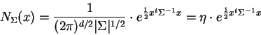
where for brevity's sake we've denoted the leading constant by ![]() .
.
A normal mixture is then defined by
![]() such that
such that
![]() , and matrix
, and matrix
![]() ,
i.e. is a positive semi-definite operator.
,
i.e. is a positive semi-definite operator. ![]() then refers
to
then refers
to
![]() . We then write
. We then write
![]() and:
and:
We will also make use of the following definite integral:
As this form is rather complex, we will denote its value
![]() in the development that follows.
in the development that follows.
Each component ![]() is further resolved into an
is further resolved into an ![]() and
and ![]() portion denoted
portion denoted ![]() and
and ![]() . By our proportionality
assumption above
. By our proportionality
assumption above
![]() and
and
![]() , from which it follows that the
eigenvectors of each
, from which it follows that the
eigenvectors of each ![]() are the same as those of
are the same as those of
![]() . We denote by
. We denote by ![]() the matrix whose columns are
these eigenvectors.
the matrix whose columns are
these eigenvectors. ![]() then denotes the ith
eigenvalue of
then denotes the ith
eigenvalue of ![]() .
We then write
.
We then write ![]() to mean
to mean ![]() , i.e. the ith component
of
, i.e. the ith component
of ![]() expressed in the Eigenbasis of
expressed in the Eigenbasis of ![]() .
.
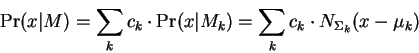
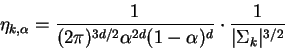
We may now compute ![]() in this Eigenbasis and enjoy the
computational and mathematical convenience of diagonal covariance
matrices:
in this Eigenbasis and enjoy the
computational and mathematical convenience of diagonal covariance
matrices:
![\begin{displaymath}
\Pr(x\vert M) =
\sum_k
\left[
c_k \eta_k
\prod_{i=1}^d e^{-\frac{1}{2} [x^k_i - (\mu_k)^k_i]^2 \lambda^k_i}
\right]
\end{displaymath}](img69.gif)
|
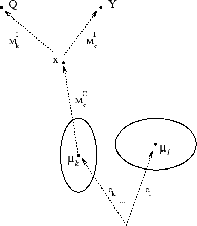
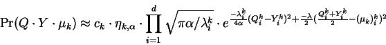
With reference to figure-1 we analyze the event
consisting of the query ![]() and a database element
and a database element ![]() being
observations of a common class representative
being
observations of a common class representative ![]() , itself
generated from
, itself
generated from ![]() . In what follows, conditioning on our
overall model of generation is implicit. We also remark that
selection of a mixture element via the
. In what follows, conditioning on our
overall model of generation is implicit. We also remark that
selection of a mixture element via the ![]() terms is assumed
to be entirely part of the
terms is assumed
to be entirely part of the ![]() process. The probability of
this event is given by:
process. The probability of
this event is given by:
So that:

Now combining the three constant ![]() factors (within the
factors (within the ![]() terms above) yields:
terms above) yields:
We then write:

Shifting to an Eigenbasis transforms the above into:
![$\displaystyle c_k \cdot \eta_{k,\alpha} \cdot \prod_{i=1}^d \int_{-\infty}^\inf...
...cdot e^{-\frac{1}{2} [Y^k_i - x^k_i]^2
\frac{\lambda^k_i}{\alpha}}
\cdot dx_i^k$](img79.gif) | |||
![$\displaystyle c_k \cdot \eta_{k,\alpha} \cdot \prod_{i=1}^d \int_{-\infty}^\inf...
... Q^k_i)^2 +
\frac{\lambda^k_i}{2\alpha} (x^k_i - Y^k_i)^2
\right]}
\cdot dx_i^k$](img80.gif) |
where it has been possible to reorder the product and integral operators because in the Eigenbasis, each dimension corresponds to an independent term. The form of EQ-1 is readily recognized and we have the result:
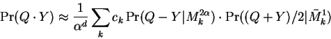
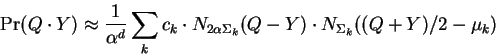
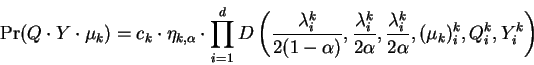
Finally, summing over the models in the mixture yields one of the main results of this paper:
which is a closed form exact solution for the joint probability we seek, given the assumptions we've made. We have therefore succeeded in dealing with the fact that class representatives are hidden, by simply integrating over all possibilities.
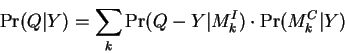
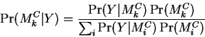
To effect classification, we select a database element ![]() maximizing
maximizing ![]() . But this conditional density is just
. But this conditional density is just
![]() and the denominator is constant for each
query. So we might as well simply maximize the joint probability.
and the denominator is constant for each
query. So we might as well simply maximize the joint probability.
Our computation of
![]() above is performed in the Eigenbasis
of each mixture component, i.e. in terms of the
above is performed in the Eigenbasis
of each mixture component, i.e. in terms of the ![]() ,
,
![]() and
and
![]() . The
. The ![]() must be computed
for each new query, but the others may be precomputed trading
a modest amount of space for considerable time savings.
must be computed
for each new query, but the others may be precomputed trading
a modest amount of space for considerable time savings.
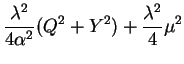
We will show that the assumption of small ![]() leads to a simpler
form of EQ-2. Our first step is to re-express each of the
four sub-terms of EQ-1 under this assumption. For brevity
we focus on a particular value for
leads to a simpler
form of EQ-2. Our first step is to re-express each of the
four sub-terms of EQ-1 under this assumption. For brevity
we focus on a particular value for ![]() and
and ![]() and therefore
omit subscripts and superscripts:
and therefore
omit subscripts and superscripts:
 |
|||
 | |||
 | |||
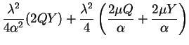 |
Before making the substitutions above, one must modify the argument
of the exponential in EQ-1 so that the second term shares
a common denominator. This is accomplished by multiplying it by
![]() in exact form. Then the approximations above may be made
and we are led to:
in exact form. Then the approximations above may be made
and we are led to:
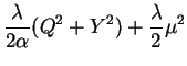
Now simplifying and rearranging constants while shifting out of the Eigenbasis and summing over mixture components leads to:
Shifting to probability notation yields the second main result of this paper:
where equality holds in the limit as ![]() approaches zero.
For clarity we've adjusted our notation slightly so that the superscript
of
approaches zero.
For clarity we've adjusted our notation slightly so that the superscript
of ![]() refers to the selected
refers to the selected ![]() factor, and a bar above
factor, and a bar above ![]() indicates that the model has a non-zero mean vector which is understood
to be subtracted.
indicates that the model has a non-zero mean vector which is understood
to be subtracted.
As ![]() approaches zero, the first probability term
becomes dominant so that
approaches zero, the first probability term
becomes dominant so that
![]() in the limit depends
only on the vector difference
in the limit depends
only on the vector difference ![]() . Moreover the sum over
components may be thought of as approximately a maximum
selector since with models such as these, a single component
usually dominates the sum. So the corresponding simplified
classification rule amounts to ``maximize over database
elements
. Moreover the sum over
components may be thought of as approximately a maximum
selector since with models such as these, a single component
usually dominates the sum. So the corresponding simplified
classification rule amounts to ``maximize over database
elements ![]() and mixture components
and mixture components ![]() the probability
the probability
![]() .'' We do not advocate this rule in part
because the assumption of vanishingly small
.'' We do not advocate this rule in part
because the assumption of vanishingly small ![]() is both
unnatural, and makes our inference of the
is both
unnatural, and makes our inference of the ![]() process from the
observed samples, even more tenuous.
We therefore suggest that EQ-3 is best applied for
small, but not vanishingly small
process from the
observed samples, even more tenuous.
We therefore suggest that EQ-3 is best applied for
small, but not vanishingly small ![]() values.
values.
The intricate mathematics of earlier sections addresses the
fact that the queries ![]() we receive and database elements
we receive and database elements
![]() we observe are not class representatives - but are
themselves the result of class and instance generation
processes.
we observe are not class representatives - but are
themselves the result of class and instance generation
processes.
Assuming instead that either the query or database elements are class representatives, one is led very quickly to simpler forms. Despite the less than satisfactory nature of this assumption, we present them because of their simplicity, and because they were the starting point of the author's work. In a sense, the complex earlier sections are the author's attempt to deal with the conceptual problems associated with these early discoveries. It is worth noting that however flawed conceptually, these forms perform very well in limited experiments [7].
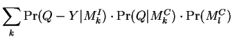
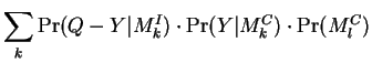
Assuming alternately that the queries ![]() are class representatives,
or that the database elements
are class representatives,
or that the database elements ![]() are, yields the two forms:
are, yields the two forms:
It is interesting to note that EQ-3 in a sense interpolates
between these two by computing
![]() .
.
If computational effort must be minimized, EQ-5 is
preferred since the ![]() can be precomputed for each
database element. Operating in an Eigenbasis is not
necessary, but as before will contribute significant
additional time savings.
EQ-4,5 are included as main results of the
paper because of their simplicity and particular computational
economy. While they do not specify the nature of the
can be precomputed for each
database element. Operating in an Eigenbasis is not
necessary, but as before will contribute significant
additional time savings.
EQ-4,5 are included as main results of the
paper because of their simplicity and particular computational
economy. While they do not specify the nature of the ![]() and
and
![]() processes, we suggest that the assumption of earlier
sections that
processes, we suggest that the assumption of earlier
sections that
![]() and
and
![]() are reasonable starting points and that the
neutral value
are reasonable starting points and that the
neutral value
![]() should be tried
first.
should be tried
first.
We now describe a variation on EQ-5 which can yield additional computational time savings. Converting to to conditional form yields:
where:
Here the database search seeks to maximize ![]() rather
than
rather
than ![]() . Over short ranges however we expect that
. Over short ranges however we expect that
![]() and therefore tolerate this
reformulation of the problem. The next practical expedient
consists of recording for each database element the component
and therefore tolerate this
reformulation of the problem. The next practical expedient
consists of recording for each database element the component
![]() for which this quantity is maximized and assuming all
others to be zero [7]. This amounts to precomputed
hard vector quantization of the database. We are then
left to deal with only a single mixture component for each
database record. Additional savings are possible
by passing to logarithms leaving what amounts to a weighted
Euclidean distance computation and addition of a constant
factor.
for which this quantity is maximized and assuming all
others to be zero [7]. This amounts to precomputed
hard vector quantization of the database. We are then
left to deal with only a single mixture component for each
database record. Additional savings are possible
by passing to logarithms leaving what amounts to a weighted
Euclidean distance computation and addition of a constant
factor.
As remarked earlier, the main results of this paper are not
metrics in the accepted mathematical sense. Metrics
![]() are usually understood to be non-negative
real valued functions of two arguments which obey three
properties: i)
are usually understood to be non-negative
real valued functions of two arguments which obey three
properties: i) ![]() iff
iff ![]() , ii)
, ii)
![]() ,
and iii)
,
and iii)
![]() . We have used the term
because it more generally means a measurement of some quantity
of interest - in our case the probability that
. We have used the term
because it more generally means a measurement of some quantity
of interest - in our case the probability that ![]() and
and ![]() are instances of some single third element
are instances of some single third element ![]() given
appropriate models for the generation of class
representatives, and instances thereof.
given
appropriate models for the generation of class
representatives, and instances thereof.
To avoid future confusion, we propose the following definition which represents a further abstraction of the setting from earlier sections:
Our development based on normal mixtures involves a two stage class
generation process. Thus we have a density ![]() , conditional
density
, conditional
density ![]() , and conditional density
, and conditional density
![]() such that:
such that:
This is easily recognized as a special case of the definition above.
Stochastic equivalence predicates in general, and our formulations in particular are certainly non-negative real valued functions of two arguments, and enjoy the symmetry property (item ii above). But that's where the agreement ends. They do not satisfy the triangle inequality (item iii) but more importantly they do not satisfy item ``i'' which we term the self-recognition axiom.
Superficially there is a problem of polarity, which is solved
by considering either
![]() or the logarithmic
form. But then would hope that
or the logarithmic
form. But then would hope that
![]() would equal
unity - having logarithm zero. Unity however is not the
value assumed and we might then consider somehow normalizing
would equal
unity - having logarithm zero. Unity however is not the
value assumed and we might then consider somehow normalizing
![]() by say
by say ![]() or some combination with
or some combination with
![]() in order to rectify the situation. Unfortunately any
such strategy is doomed because of the following observation:
Viewing
in order to rectify the situation. Unfortunately any
such strategy is doomed because of the following observation:
Viewing ![]() as a free variable,
as a free variable,
![]() does not
necessarily assume its maximal value when
does not
necessarily assume its maximal value when ![]() .
3
.
3
This is at first a deeply troubling fact. Other investigators have employed distance functions which do not obey property iii above, and symmetry is sometimes abandoned. But self-recognition is somehow sacred. If our distance functions are in any sense an improvement, then we are presented with:
The ``self recognition'' paradox: the better distance function
may have the property that there are querieswhich do not
recognize themselves, i.e. even if
some other elementmay be preferred.
The paradox is resolved through better understanding the
quantity that the stochastic equivalence predicates measure with particular emphasis on
the assumption that ![]() and
and ![]() represent independent
observations.
represent independent
observations.
Recall that our model imagines ![]() and
and ![]() to be noisy
observations (instances) of some hidden object
to be noisy
observations (instances) of some hidden object ![]() , which may
be thought of as a platonic ideal. We also assume a
probability model4 for these ideals
, which may
be thought of as a platonic ideal. We also assume a
probability model4 for these ideals ![]() and a second model for the
generation of noisy observations of
and a second model for the
generation of noisy observations of ![]() . It is crucial to
observe that we also assume that the observation of
. It is crucial to
observe that we also assume that the observation of ![]() and
and
![]() are independent events. So having fixed
are independent events. So having fixed ![]() , and assuming that
, and assuming that
![]() is a somewhat noisy image of it with correspondingly low
probability
is a somewhat noisy image of it with correspondingly low
probability ![]() , the fact that
, the fact that ![]() may equal
may equal ![]() is not a
remarkable event and the probability of observing them both
conditioned on
is not a
remarkable event and the probability of observing them both
conditioned on ![]() is just
is just ![]() .
.
An example serves to better illustrate this point. Imagine
listening to music broadcast by a distant radio station. If
the same song is played twice, we hear two different noise
corrupted versions of the song. A reasonable but crude model
of music would expect locally predictable signals and would
therefore assign somewhat higher probability to the original
than to noisy versions. Now let ![]() be the original recording
of a song as broadcast from the station, and suppose that we
hear on a particular day a very noisy version
be the original recording
of a song as broadcast from the station, and suppose that we
hear on a particular day a very noisy version ![]() . Further
suppose that over time we have assembled a database of music
as recorded from this distant station. Assume the database
contains a version
. Further
suppose that over time we have assembled a database of music
as recorded from this distant station. Assume the database
contains a version ![]() of
of ![]() recorded on an earlier day on
which favorable atmospheric conditions prevailed resulting in
an almost noiseless version. Now given any reasonable model
for noise we would expect that the probability of
recorded on an earlier day on
which favorable atmospheric conditions prevailed resulting in
an almost noiseless version. Now given any reasonable model
for noise we would expect that the probability of ![]() given
given
![]() to be far less than the probability of
to be far less than the probability of ![]() given
given ![]() . But
then:
. But
then:
whence a search of the database using our
stochastic equivalence predicate would choose ![]() even if
even if ![]() itself is present.5
itself is present.5
To recapitulate: stochastic equivalence predicates attempt to measure the probability that two observations have a common hidden source not how much they differ. This objective leads to distance functions which do not have the self-recognizing property but are nevertheless better to the extent that their constituent models correspond to nature.
We now endeavor to illuminate the relationship between our
model and the argument above to the traditional nearest
neighbor outlook6. To begin consider
EQ-4 which was derived under the assumption that
the queries are class representatives (not noisy observations
thereof). Notice that
![]() is maximized when
is maximized when
![]() and that the other two terms do not depend on
and that the other two terms do not depend on ![]() . So
this form does have the self recognizing property. The
same is not necessarily true of EQ-5.
. So
this form does have the self recognizing property. The
same is not necessarily true of EQ-5.
One may then reconcile the conventional nearest neighbor outlook with this paper's framework by adding the assumption that the queries are class representatives. Unfortunately for some problems this is almost certainly false and the conventional nearest neighbor approach is simply flawed. Another approach one might take is to define two conditional models, one for queries and one for database elements since the nearest neighbor approach seems to implicitly assume that queries are in essence noiseless observations of class representatives. We will however not develop this approach in this paper.
So to the extent that we can accurately model platonic ideals and observation noise, we submit that that stochastic equivalence predicates are asking the right question and conventional metrics the wrong one.
We view our approach as a form of unsupervised metric learning - although as we have seen, we do not obtain a metric in the mathematical sense. From the statistical viewpoint our approach is a way to obtain a joint density from a simple density plus strong additional assumptions.
If the mixture contains a single component, our methods correspond to the well known heuristic technique of employing weighted Euclidean distances - with the weights inversely proportional to the feature variances.7
If the number of elements in the mixture is equal to the
number of classes, then our approach tends (at least
conceptually) to the traditional Mahalanobis distance method
given sufficient data. We will now sketch the intuition behind
this observation. If many examples of each class are
available, then the mixture density learned will plausibly
have a term for each class. Focusing on EQ-5
because it is easiest to interpret, and on a database element
![]() which lies very near to the mean of its class, we might
hope that
which lies very near to the mean of its class, we might
hope that ![]() is greatest for the class to which
is greatest for the class to which
![]() belongs - and imagine it to be unity. Also
belongs - and imagine it to be unity. Also
![]() since we've assumed
since we've assumed
![]() . So we might reasonably expect a nearest neighbor
search of the
. So we might reasonably expect a nearest neighbor
search of the ![]() which are near to their class means to
yield roughly the same result as a traditional Mahalanobis
Distance method. Finally we might hope the the presence of
other members of the class in the database will in general help
- not hurt classifier performances.
which are near to their class means to
yield roughly the same result as a traditional Mahalanobis
Distance method. Finally we might hope the the presence of
other members of the class in the database will in general help
- not hurt classifier performances.
If the number of elements in the mixture is intermediate between these two extremes, the elements represent super-classes of those we're interested in. Of primary interest we feel, is this intermediate region in which a more effective distance function might be discovered by uncovering hidden structure in the data.
As the database grows one may increase the number of mixture elements so that our scheme spans the entire spectrum from a starved starting point in which one can expect to have only a single representative of each class, to the data-rich extreme in which many exist.
Regarding our ![]() parameter, we remark that it should
be thought of as domain dependent. However values very near
to zero create conceptual difficulties8, since they correspond to
parameter, we remark that it should
be thought of as domain dependent. However values very near
to zero create conceptual difficulties8, since they correspond to ![]() processes which generate vanishingly small variations on a
class representatives. The problem is that our assumption
that we can infer anything of the
processes which generate vanishingly small variations on a
class representatives. The problem is that our assumption
that we can infer anything of the ![]() process as
process as ![]() approaches zero becomes increasingly tenuous.
approaches zero becomes increasingly tenuous.
In this paper we've presented only one approach to inference. Strong
assumptions were made so that a closed form solution would result.
More sophisticated approaches represent an interesting area
for future work. Given some prior knowledge of the ![]() and
and ![]() processes
one might strive to compute posteriori structures. Or one might have access to
a supply of instance pairs known to have been generated by the same
class representative - and somehow use this information to advantage.
Finally this work might be extended to the supervised case
in which class or superclass labels are available.
processes
one might strive to compute posteriori structures. Or one might have access to
a supply of instance pairs known to have been generated by the same
class representative - and somehow use this information to advantage.
Finally this work might be extended to the supervised case
in which class or superclass labels are available.
In this section we remark on several matters of practical importance and suggest simple solutions. They relate the problems associated with estimating the parameters of complex models such as the multidimensional normal mixtures we rely on - and to our choice of Gaussian densities.
In our development so far, we have assumed that the number ![]() of
elements in the normal mixture was somehow given. In practice
it is difficult to decide which value is best. The approach we prefer
begs this question by instead starting with a prior on a range
of possible values and combining the results of all the models.
If
of
elements in the normal mixture was somehow given. In practice
it is difficult to decide which value is best. The approach we prefer
begs this question by instead starting with a prior on a range
of possible values and combining the results of all the models.
If ![]() denotes a mixture model with
denotes a mixture model with ![]() elements, then this
amounts to computing:
elements, then this
amounts to computing:
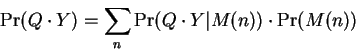
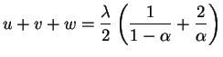
In one experiment [7], this blended distance
performed as well as the single best value. Assuming a flat
prior and passing to logarithms, we remind the reader that
this blend is well approximated by the ![]() operation,
i.e. by choosing the shortest code-length.
operation,
i.e. by choosing the shortest code-length.
Our discussion above has avoided the details of learning the necessary mixture density, and in fact not mentioned the delicate matter of estimating the parameters of a single multivariate normal density given little data. We therefore comment that in practice one may use the well known Expectation Maximization (EM) method to obtain a (locally) maximum-likelihood mixture model. In this case as well as with a single density, some form of statistical flattening is advisable if little data is available. In this section we briefly describe practical techniques for dealing with this issue.
One convenient statistical device amounts to believing the
variances before the covariances. One multiplies the off-diagonal
entries of ![]() by some scaling factor
by some scaling factor ![]() . Avoiding
unity has the additional advantage of preventing ill-conditioned
matrices (assuming none of the variances are near zero). This
is discussed in greater detail in [7].
. Avoiding
unity has the additional advantage of preventing ill-conditioned
matrices (assuming none of the variances are near zero). This
is discussed in greater detail in [7].
It should be mentioned that given enough data one might attempt to
assign different values of ![]() to each mixture component. Intuitively
this makes sense since some components may have many members while
others have relatively few. Those with many members might be expected
to work well with
to each mixture component. Intuitively
this makes sense since some components may have many members while
others have relatively few. Those with many members might be expected
to work well with ![]() values closer to unity.
values closer to unity.
It is worthwhile noting that in cases where the feature vectors have finite support, e.g. each feature is contained in say the unit interval, one should instead consider estimating the parameters of a mixture of multi-dimensional beta densities. Liporace [8] demonstrates that this introduces only small complications for a somewhat general class of densities.
Consider a two dimensional distribution made up of two zero mean normal densities, of equal probability, but with covariance matrices which result in ellipsoidal contours that are very different. In particular, the principal axis of each are 90 degrees apart. Also, one has a small minor axis, while the other is closer to circular. Assume that each corresponds to items of a given class. Then it is not too great a challenge for mixture density estimators to discover this structure without the labels. The stochastic equivalence predicates described in this paper will then give rise to a very different decision boundary than would result from say simple Euclidean distance. This example also illustrates that the mixture components discovered might have identical means but very different covariance matrices.
The example above might of course have been dealt with using other methods since it has a simple discrete two class structure. More interesting examples would exhibit a continuous class structure corresponding to some continuous parameter such as age. Here our discrete mixture would attempt to approximate this continuous variation by covering various regions with different normal densities.
Encoder nets9 [9] are feed-forward neural networks which include a highly constricted layer - forcing the network to somehow compress/encode its inputs and then decompress/decode them to arrive at an output which approximates the inputs. This well known design approach is an effective way to avoid over-training.
Our focus is on the constricted layer only. Each input vector presented to the network gives rise to some pattern of activations at this layer. Considering this pattern as real vector, we then suggest that the methods of this paper can be applied to learn a distance function for this space of activation patterns.
So given two inputs ![]() to the network giving rise to encodings
to the network giving rise to encodings ![]() ,
, ![]() ,
we might compute a distance between them. This distance can then be used
to effect classification via nearest neighbor search of some labeled dataset.
Thus after training, the final stages of the network can essentially be
discarded.
,
we might compute a distance between them. This distance can then be used
to effect classification via nearest neighbor search of some labeled dataset.
Thus after training, the final stages of the network can essentially be
discarded.
There is some evidence that this general approach is effective. In [10] a neural net the authors call LeNet-4 was trained to achieve 1.1% classification error for the problem of handwritten digit recognition. The authors realized that a particular 50-unit layer might be thought of as a feature vector, and built a pattern classifier using the Euclidean distance metric. The resulting system achieved the same 1.1% error level. What isn't clear from their work is whether the more complex forms of this paper could have improved performance further. If the activation vector is described well by a single normal density with covariance proportional to the unit matrix, then we would expect Euclidean distance to be essentially optimal. If however structure is evident in a sample of the space of such vectors, it may be that our methods can be used to advantage.
We speculate that it might also be possible to influence training so as to prefer networks having simple statistics in their encoder layer. In addition to simplifying later distance computations, this might have a positive impact on the network itself.
Common front end signal processing in speech recognition systems reduces signal windows to feature vectors of dimension 10-20. It would be interesting to explore the application of unsupervised metric learning in general, and our stochastic equivalence predicates in particular, to this setting since the data are not conveniently labeled. Many other applications might benefit from our techniques. These include almost any problem for which nearest neighbor search is somewhat effective.
Common front end signal processing in speech recognition systems reduces signal windows to feature vectors of dimension 10-20. It would be interesting to explore the learning of stochastic equivalence predicates for this space since the data are not conveniently labeled. Many other applications might benefit from our techniques. These include almost any problem for which nearest neighbor search is somewhat effective.
The author thanks Ingemar Cox and David Jacobs for helpful discussions. Our joint work on face recognition from feature vectors [11] provided much needed concrete examples from which the author drew the intuition needed to complete this work. This work now continues with the authors above as well as Joumana Ghosn [7]. I thank Adam Grove and Steve Omohundro for helpful discussions and comments on earlier drafts. I also thank Eric S. Ristad. Our joint work on handwriting recognition and stochastic modeling contributed greatly to my thinking in this area.
This document was generated using the LaTeX2HTML translator Version 2K.1beta (1.47)
Copyright © 1993, 1994, 1995, 1996,
Nikos Drakos,
Computer Based Learning Unit, University of Leeds.
Copyright © 1997, 1998, 1999,
Ross Moore,
Mathematics Department, Macquarie University, Sydney.
The command line arguments were:
latex2html -split 0 -image_type gif -nonext_page_in_navigation -noprevious_page_in_navigation -up_url ../main.html -up_title 'Publication homepage' -numbered_footnotes mlnm.tex
The translation was initiated by Peter N. Yianilos on 2002-07-03

![\begin{displaymath}
\Pr(Q \cdot Y ) =
\sum_k \left[
c_k \cdot \eta_{k,\alpha...
...k_i}{2\alpha},
(\mu_k)^k_i,
Q^k_i,
Y^k_i
\right)
\right]
\end{displaymath}](img82.gif)