Significantly Lower Entropy Estimates for Natural DNA Sequences

David Loewenstern*
NEC Research Institute, 4 Independence Way, Princeton, NJ 08540
Phone: 609-951-2798 Fax: 609-951-2483
Email: loewenst@paul.rutgers.edu
and
Peter N. Yianilos
NEC Research Institute, 4 Independence Way, Princeton, NJ 08540
and
Department of Computer Science Princeton University, Princeton, New Jersey 08544
Email: pny@research.nj.nec.com

Submitted: November 10, 1996

Abstract:

If DNA were a random string over its alphabet $\{A,C,G,T\}$, an optimal code would assign $2$ bits to each nucleotide. DNA may be imagined to be a highly ordered, purposeful molecule, and one might therefore reasonably expect statistical models of its string representation to produce much lower entropy estimates. Surprisingly this has not been the case for many natural DNA sequences, including portions of the human genome. We introduce a new statistical model (compression algorithm), the strongest reported to date, for naturally occurring DNA sequences. Conventional techniques code a nucleotide using only slightly fewer bits (1.90) than one obtains by relying only on the frequency statistics of individual nucleotides (1.95). Our method in some cases increases this gap by more than five-fold (1.66) and may lead to better performance in microbiological pattern recognition applications.

One of our main contributions, and the principle source of these improvements, is the formal inclusion of inexact match information in the model. The existence of matches at various distances forms a panel of experts which are then combined into a single prediction. The structure of this combination is novel and its parameters are learned using Expectation Maximization (EM).

Experiments are reported using a wide variety of DNA sequences and compared whenever possible with earlier work. Four reasonable notions for the string distance function used to identify near matches, are implemented and experimentally compared.

We also report lower entropy estimates for coding regions extracted from a large collection of non-redundant human genes. The conventional estimate is 1.92 bits. Our model produces only slightly better results (1.91 bits) when considering nucleotides, but achieves 1.84-1.87 bits when the prediction problem is divided into two stages: i) predict the next amino acid based on inexact polypeptide matches, and ii) predict the particular codon. Our results suggest that matches at the amino acid level play some role, but a small one, in determining the statistical structure of non-redundant coding sequences.

Keywords:DNA, Information Theoretic Entropy, Expectation Maximization (EM), Data Compression, Context Modeling, Time Series Prediction.

Introduction

The DNA molecule encodes information which by convention is represented as a symbolic string over the alphabet $\{A,C,G,T\}$. Assuming each character (nucleotide) is drawn uniformly at random from the alphabet, and that all positions in the string are independent, we know from elementary information theory [Cover and Thomas, 1991,Bell et al., 1990] that an optimal code will devote 2 bits to representing each character. This is the maximum entropy case. DNA may be imagined to be a highly ordered, purposeful molecule, and one might therefore reasonably expect statistical models of its string representation to produce much lower entropy estimates, and confirm our intuition that it is far from random. Unfortunately this has not been the case for many natural DNA sequences, including portions of the human genome.

One example is the human retinoblastoma susceptibility gene containing $180,388$ nucleotides, and referred to as HUMRETBLAS. The alphabet members do not occur with equal frequency in this string, and accounting for this yields an entropy estimate of roughly $1.95$ bits. This is perhaps not surprising since such single character models are the weakest in our information theory arsenal. A logical next step taken by several investigators, focuses instead on higher order entropy estimates arising from measurements of the frequencies of longer sequences. For natural languages (e.g. English) this step typically leads to significantly lower entropy estimates. But the best resulting estimate for HUMRETBLAS is roughly $1.90$ bits [Mantegna et al., 1993], still not impressively different from our $2$-bit random starting point. This may be something of a surprise, since such models reflect such known DNA structure as $\%(C+G)$ composition and CG suppression. But these known effects have little impact on the entropy of DNA sequences as a whole.

One may view DNA as a time series, and these higher order models as predictors of the next nucleotide based on its immediate past. With this interpretation the simple $1.95$ bit model relies on none of the past. The $1.90$ bit result is then even more surprising since it implies that knowledge of the immediate past reduces the entropy estimate by a mere $0.05$ bits.¹ Data compression techniques such as Lempel-Ziv (LZ) coding [Ziv and Lempel, 1977] may be viewed as entropy estimators, with LZ corresponding to a model that predicts based on a historical context of variable length. It ``compresses'' HUMRETBLAS to $2.14$ bits per character², which is actually worse than the flat random model we started with. The authors' earlier efforts implemented other advanced modeling techniques but failed to obtain estimates below approximately $1.88$ bits.

In this paper we describe a new statistical model, the strongest we are aware of, for naturally occurring DNA sequences. The result is lower entropy estimates for many sequences. Our experiments include a wide variety of DNA, and in almost all cases our model outperforms the best earlier reported results. For HUMRETBLAS, the result is approximately $1.7$ bits per character -- $0.25$ bits improved from our $1.95$ bit starting level. The standard higher order estimate of $1.90$ bits is only $0.05$ bits lower, so in this sense our result represents a five-fold improvement. In every case our model outperforms the most common techniques. These results are significant because of our model's consistent and frequently substantial advantage over earlier methods.

So far we have described the quest for lower entropy estimates as a rather pure game, i.e. to predict better an unknown nucleotide based on the rest of the sequence. There are both conceptual and practical reasons to believe that this is an interesting pursuit and that our experimental results are of some importance. Conceptually, the pursuit of better models for data within some domain corresponds rather directly to the discovery of structure in that domain. That is, we model so that we can better understand. Practically, statistical modeling of DNA has proven to be somewhat effective in several problem areas, including the automatic identification of coding regions [Lauc et al., 1992,Cosmi et al., 1990,Cardon and Stormo, 1992,Farach et al., 1995,Krogh et al., 1994], and in classifying unknown sequences into one of a discrete number of classes. The success of such methods ultimately rests on the strength of the models they employ.

In section 2 we discuss the interpretation of entropy estimates obtained by methods such as ours, and by other approaches such as data compressors. The definition of entropy in the context of DNA nucleotide prediction is made more precise, and we discuss entropy estimates for coding regions.

A detailed exposition of our model is presented in section 3, but we first introduce and motivate it here in general terms. Conventional fixed-context models focus on a trailing context, i.e. the immediately preceding nucleotides. Longer contexts reach farther into the past, and might reasonably be expected to result in stronger models. However as context length increases, it becomes increasingly unlikely that a given context has ever been seen. This problem has led to the development of variable length context language models [Bell et al., 1990], which use long contexts when enough earlier observations exists, and otherwise use shorter ones. Since as earlier noted, the short-term behavior of many natural DNA sequences is so nearly random, these more advanced variable length schemes do not push farther into the past, except in the unusual event of a long exact repeat.

The basic idea behind our model is to push farther into the past by relaxing the exact-match requirement for contexts. Our formalization of this idea in section 3 is one of the main contributions of this paper.

The metric for determining quality of match is primarily a simple Hamming distance, but in the interests of exploring the use of additional biological knowledge, three other metrics were evaluated in section 6. We also describe a two-stage model for coding regions in which an amino acid is first predicted based on earlier amino acids, followed by the prediction of a particular codon. Section 6 concludes with a discussion that suggests why the high entropy levels observed for coding regions may not be so surprising after all.

Entropy Estimation and Data Compression

The term entropy estimate can be somewhat vague. This section continues our introduction of the term by clarifying its various senses as they relate to DNA, and its relationship to data compression and prediction. We include the section in part to answer some of the most frequently asked basic questions about this work. Our discussion will first focus on the sense of entropy that corresponds to a stochastic process. Later, we describe another equivalent sense more suited to sequences of finite extent. The entropy rate of a stochastic process $\{X_t\}$ is defined as:

$$\lim_{t \rightarrow \infty} \frac{1}{t} H(X_1,X_2,\ldots,X_t)$$ (1)

where this limit need not in general exist, and $H$ denotes the information theoretic entropy function (see [Cover and Thomas, 1991].) Given full knowledge of the process, and the limit's existence, the entropy rate is a well-defined attribute of the process. But we know very little of the process underlying the generation of natural DNA, and can merely observe the outcome, i.e. the nucleotide sequence. Given a predictive model ${\cal X}$, and a long DNA sequence $\{x_t\}$, we are therefore content to consider:

$$\lim_{t \rightarrow \infty} \frac{1}{t} \log_2 \Pr(x_t\vert x_1,\ldots,x_{t-1},{\cal X})$$ (2)

This may be thought of as the average bits per symbol required to code increasingly long observation sequences. If our model matches Nature perfectly, Nature's process is in some sense well-behaved³, and our sequence is of infinite length, then this limit matches the entropy rate. Of course: i) our model does not match Nature, ii) there is no reason to believe Nature is in the required sense well-behaved, and iii) we can observe only finite DNA sequences. It is in this sense that one is computing an entropy estimate when an imperfect model is applied to a finite empirically observed sequence.

Given a data compression program, Equation 2 may therefore be approximated by dividing the number of bits output by the number of symbols (nucleotides) input. We will refer to computations like this as purely compressive entropy estimates. Most existing compression algorithms, when applied to natural data, do in fact frequently approach a limit in bits/character -- their estimate of the source's entropy. Unless the sequence being compressed is very long, the purely compressive estimate then overstates the actual entropy. One might then focus only on the code-lengths near the end of the sequence. The risk however is then that the end might just happen to be more predictable and not reflect the overall entropy. For example, the end might, in the case of DNA, contain many long exact repeats of earlier segments. This suggests our second approach, that of cross-validation entropy estimates. Here the sequence is first partitioned into $N$ equal size segments. The entropy of each segment is then computed by coding it having first trained the model using the remaining segments. The reported entropy estimate is the average of these $N$ estimates. One can imagine that each of these estimates moves one segment to the end of the sequence, codes it, and averages code-lengths for the final segment only. As $N$ increases, the individual cross-validation estimates may be plotted to visualize the instantaneous entropy rate as a function of position in the sequence. Several of these plots are presented in section 5.

In what follows, we will switch without harm between a compressive viewpoint, that of stochastic prediction in which the objective is to predict the next nucleotide, and generative stochastic modeling in which one imagines the data to emanate from a particular process. This is possible because a generative process gives rise to a prediction, and a prediction can be converted to a code via arithmetic coding. Starting from a data compressor, we can think of the bits output for a single input symbol, as $\log_2$ of the probability that a corresponding predictor will predict, or generator will generate that symbol⁴.

The models discussed so far in this paper introduce only one kind of domain knowledge: that natural DNA sequences include more near repetitions than one expects at random. Part of the reason that so little effort has been devoted to more advanced models that incorporate complex domain knowledge, is that models of the ignorant variety do a very good job of modeling other natural sequences. For example, Shannon's work estimated the entropy of English text to be roughly $1.3$ bits per character (see discussion in [Bell et al., 1990]). Random text over a 27 letter alphabet (A-Z and space) corresponds to $4.8$ bits. Today's statistical models, with no specific knowledge of English syntax or semantics, can achieve roughly $2$ bits.

Returning to the question that opened our discussion, we submit that the essential cause of our surprise is that simple statistical models, which perform so well in other cases, fail to discover significant structure in DNA. Our work demonstrates that DNA is more predictable than had previously been established, but falls far short of the compression levels easily achieved for natural language. This suggests that local structure parallel to ``words'' and ``phrases'' is largely missing in DNA, even when the exact match requirement is relaxed.

As to ``what entropy level we expect and why'', we believe that the question ultimately comes down to one of quantifying the magnitude of the functional degeneracy of polypeptides. That is, how many different sequences are essentially equivalent functionally? If this degeneracy turns out to be large, then DNA is to its function, as an acoustic waveform is to human speech. That is, small local distortions do little to alter the overall message. This is discussed further in Section 6.

Algorithms

In this section we further motivate our model and then describe it in formal terms.

That natural DNA includes near repeats is well known, and in [Herzel, 1988] the statistics of their occurrence are discussed. We measure nearness using ordinary Hamming distance, i.e. the number of positions at which two equal length strings disagree. Given a target string of length $w$, it is then natural to wonder how many $h$-distant matches exist in a string of length $\ell$. As remarked earlier, DNA seems very nearly random over short distances. Assuming uniform randomness it is easily shown that we expect to see $\ell \cdot 3^h/4^w \cdot \mbox{\footnotesize$\ \left( \!\!\! \begin{array}{c} w \\ h \end{array} \!\!\! \right)$}$ $h$-distant matches. Natural DNA sequences depart markedly from this behavior, providing one part of the motivation for our model. For example (table 1), using HUMRETBLAS, which consists of $180,388$ nucleotides, and a randomly chosen substring of length $w=20$ from the first $\frac{1}{8}$ of the sequence, one expects $8.61 \times 10^{-6}$ Hamming distance $h=1$ matches in the last $\frac{7}{8}$ of the sequence under the random model. We actually see $0.143$ where again, this is an average over all length $20$ targets in the last $\frac{7}{8}$ of HUMRETBLAS. When such matches exist, examination of the following nucleotide yields a prediction that is correct $83.77\%$ of the time. That these matches, when present, lead to good predictions is a second motivating factor. Unfortunately such Hamming distance $1$ matches occur for only $7.2\%$ of the positions in HUMRETBLAS, so alone, this effect is unlikely to lead to much better predictions on average. But if one again refers to table 1, roughly $1/3$ of the positions have an earlier match at distance $4$ - and at even this distance, predictions based on past matches are correct $45.91\%$ of the time. The potential effectiveness of predictions based on matches at all distances is our final motivating factor. The objective, then, is to combine these weak information sources to form a prediction. Also, a version of table 1 may be made for multiple windows. Our model combines all of this information and makes a single prediction. The use of near matches for prediction is certainly consistent with an evolutionary view in which Nature builds a genome in part by borrowing mutated forms of her earlier work.

One may view each row of table 1 (really each Hamming distance) as corresponding to a predictive expert, $\Pr(b\vert h=i,w=k,\mbox{\em past})$. The prediction of the Hamming distance $2$ expert, $\Pr(b\vert h=2,w=20,\mbox{\em past})$ is formed by examining all past matches exactly this distance from our trailing context window, and capturing the distribution of following nucleotides by maintaining a simple table of counters. The simplest way to combine these experts is by a fixed set of weights that sum to one.

But suppose that while trying to predict a particular nucleotide $b$ using $w=20$, our past experience includes no Hamming distance $0-3$ matches, i.e. the closest past window is distance $h=4$. This information is known before we see the to-be-predicted nucleotide and may therefore influence the prediction. In particular it makes no sense to give any weight to the opinions of the first three experts -- in fact their opinion is not even well-defined in this case. Only the $17$ experts corresponding to Hamming distances $4-20$ are relevant. We're then interested in properly weighting them conditioned on the assumption that the closest match we've seen lies at distance $4$. In what follows we will refer to this value as first Hamming, $f$. Finally, since we don't know a priori how window size will influence the prediction, our model is formed at the uppermost level by a mixture of models, each considering a fixed window size from some fixed prior set.

We denote by $b$ the discrete random variable representing the nucleotide (base-pair) to be predicted. Its four values are $b=1,2,3,4$ and correspond to $A,C,G,T$. By $w$ we denote the positive integer random variable corresponding to the length of our trailing context window. The set of values it may assume is parameter of the model, defined by specifying non-zero prior probabilities for only a finite subset of the positive integers. For example, allowing $w=2,4,6,8$ considers context windows of these four lengths. Next, $f$ denotes the first Hamming distance to be considered. It may assume values $0,\ldots,w$. By $h$ we denote the index of each Hamming distance expert. So $h$ lies in the range $0,\ldots,w$. Finally, we use $\mbox{\em past}$ to represent our modeling past, i.e. the DNA that we have either already predicted, or have set aside as reference information.

Given a fixed window size $w=k$, and distance $h=i$, there is a natural prediction $\Pr(b\vert h=i,w=k,\mbox{\em past})$ formed by locating all distance $i$ matches in the past to the trailing context of length $k$, and then using the distribution of nucleotides that follow them. This is a single expert as described above. This prediction is independent of $f$ so $\Pr(b\vert h=i,w=k,\mbox{\em past}) = \Pr(b\vert h=i,f=j,w=k,\mbox{\em past})$. Our prediction $\Pr(b\vert\mbox{\em past})$ arises from the joint probability $\Pr(b, h, f, w\vert\mbox{\em past})$ by summing over the hidden variables $h,f,w$ as follows:

$$\Pr(b\vert\mbox{\em past}) = \sum_{i,j,k} \Pr(b\vert h=i,f=j,w=k,\mbox{\em past}) \cdot \Pr(h=i,f=j,w=k,\mbox{\em past})$$ (3)

The final term is then expressed as a product of conditionals:

$$\Pr(h=i,f=j,w=k,\mbox{\em past}) = \Pr(h=i\vert f=j,w=k,\mbox{\em past}) \cdot \Pr(f=j\vert w=k,\mbox{\em past}) \cdot$$

$$\Pr(w=k\vert\mbox{\em past}) \cdot \Pr(\mbox{\em past})$$ (4)

In this expression $\Pr(\mbox{\em past}) = 1$ and $\Pr(f=j\vert w=k,\mbox{\em past}) = 1$ for $j$ equal to the distance of the closest match to our trailing context window of length $k$, in the $\mbox{\em past}$. At all other values $\Pr(f=j\vert w=k,\mbox{\em past})=0$. That is, $\Pr(f=j\vert w=k,\mbox{\em past})$ is a boolean function $f(j,k,\mbox{\em past})$. Next, we assume $w$ is independent of the past in our model, so $\Pr(w=k\vert\mbox{\em past}) = \Pr(w=k)$ and consists of a vector of fixed mixing coefficients that select a window size. Introducing a dependency here may improve the model and represents an interesting area for future work. Finally, in our model $\Pr(h=i\vert f=j,w=k,\mbox{\em past})$ is also independent of the past and consists of a fixed vector of $k-j+1$ mixing coefficients that select a Hamming distance given the earlier choice of a window size $k$, and observation that the nearest past match is at distance $j$. We then have:

$$\Pr(b\vert\mbox{\em past}) = \sum_{i,j,k} \Pr(b\vert h=i,w=... ...(h=i\vert f=j,w=k) \cdot f(j,k,\mbox{\em past}) \cdot \Pr(w=k)$$ (5)

The first term in the summation is recognized as a single expert, the second selects an expert based on $f$ and $w$, the third deterministically selects a single $f$ value, which receives probability $1$, and the final term selects a window size. The first and third terms are determined entirely from the current context and the past; the second and fourth terms are selection parameters that must be tuned during a learning process.

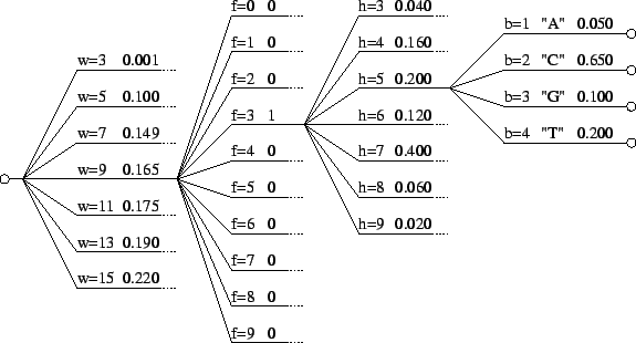
The model may also be viewed generatively (reading from left to right) as depicted in figure 1. In this example a window size $w$ is first chosen from the set $\{3,5,7,\ldots,15\}$. The probability of each choice is shown beside it. Notice that they, and all choices at each node in the diagram, sum to unity. In the figure, $w=9$ is chosen and the next choice is deterministic. Here we've assumed that the closest match to our trailing context of length $9$ is distance $3$ away. Now given $w=9$ and $f=3$ we choose $h \in 3,\ldots,9$ with the probabilities shown. Here we've assumed that $h=5$ is chosen. Finally, given all the earlier choices, we generate a nucleotide $b$ according to probabilities shown.

Figure 1: An illustration of the generative branching process that corresponds to the predictive model of this paper.

We refer again to figure 1 to clarify the model's parameter structure. The probabilities associated with the choice of $w$ are parameters, as are those associated with the choice of $h$ for each $f$ and $w$. But recall that the probabilities on each $f$ arc in the graph are computed and are not therefore parameters. Similarly the probabilities associated with $b$ are not parameters. They too are computed and represent the opinion of a single expert as described earlier. Thus for the figure shown there are $7$ parameters for $w$, and $4+6+\ldots+16 = 70$ associated with $h$, for a total of $77$. Other parameters include our selection of window sizes to consider, and several explained below having to do with the learning algorithm.

The learning task before us is to estimate these parameters by examining the training set. Our algorithm is an application of the Baum-Welch algorithm for Hidden Markov Models [Baum and Eagon, 1967,Baum et al., 1970,Baum, 1972,Poritz, 1988], and may also be viewed as an instance of Expectation Maximization (EM), a later rediscovery [Dempster et al., 1977,Redner and Walker, 1984] of essentially the same algorithm and underlying information theoretic inequality.

The Baum-Welch algorithm is an optimization technique which locally maximizes the probability of generating the training set from the model by adjusting parameters. A global optimization method would be expected to yield better results in general. In the general case, however, the problem of globally optimizing directed acyclic graph-based models is known to be NP-complete (see [Yianilos, 1997, p. 32]). Our model fits within this class but we have not considered the complexity of its optimization. It is known, however, to exhibit multiple local optima.⁵

In the case of our model, the parameters are the probability associated with $w$, $\Pr(w=i)$, and the probability associated with $h$, $\Pr(h=i\vert f=j,w=k)$. Before learning begins, these parameters are initialized in our implementation to the flat (uniform) distribution. Examples from the training set are now presented repeatedly, and these parameters are reestimated upon each presentation -- climbing away from their starting values towards some set of values that locally maximize the log likelihood of the training set.

The training set consists of a series of prediction problems: predict a given nucleotide $b$ using its trailing context and some past reference DNA. For the experiments of this paper, we select positions to be predicted at random from the training DNA. The rest of the sequence then serves as reference when searching for near-matches. Because of the simple tree-like branching structure of our model, the reestimation formulae are particularly simple and natural. Accumulated expectations are first computed by:

$$E(\Pr(w=k)) = \sum_b \frac{\Pr(b,w=k\vert\mbox{\em past})}{\Pr(b\vert\mbox{\em past})}$$ (6)

where the probabilities are assumed to be conditioned on the model's current parameter set, and the summation is over our randomly chosen positions to be predicted. The reestimated window selection probabilities are then:

$$\overline{\Pr(w=k)} = \frac{E(\Pr(w=k))}{\sum_\ell E(\Pr(w=\ell))}$$ (7)

Expectations for $h$ are accumulated according to:

$$E(\Pr(h=i\vert f=j,w=k)) = \sum_b \frac{\Pr(b,w=k,f=j,h=i\vert\mbox{\em past})}{\Pr(b\vert\mbox{\em past})}$$ (8)

The reestimated conditional Hamming distance selection probabilities are then:

$$\overline{\Pr(h=i\vert f=j,w=k)} = \frac{E(\Pr(h=i\vert f=j,w=k))}{\sum_\ell E(\Pr(h=\ell\vert f=j,w=k))}$$ (9)

This new parameter set $\{\overline{\Pr(w=k)},\overline{\Pr(h=i\vert f=j,w=k)} \}$ must increase the likelihood of the training set under the model. Performing the steps above once corresponds to one EM iteration. Each iteration will continue to improve the model unless a local maximum is reached. In section 5 we will study the effect of these iterations on the performance of our model, and also examine the model's sensitivity to other parameters.

At the conclusion of each reestimation step above, the reestimated vector is normalized to sum to unity. This operation is also performed when an expert converts counts derived from earlier matches into a stochastic prediction for the next nucleotide. In both places it is possible for one or even all vector locations to be zero. The result is then one or more zero probabilities after normalization. If the entire vector is zero, the normalization operation is of course no longer even well-defined. To ensure that our system deals only with finite code-lengths, and to handle the all-zero case simply, we, as a practical expedient, add a small constant, $1 \times 10^{-10}$, to each vector position before normalization. We stress that this is not done for the same reason that one might use Laplace's rule (add one to event counts) to flatten the prediction of a simple frequency-based model. Such techniques are basically a remedy for data sparseness. We require no such flattening since our model is itself a mixture of many experts, including some for which plenty of data is available. Experiments confirm our intuition that additional Laplace-style flattening is in fact harmful.

We conclude by sketching the operation of a fully on-line model. Rather than performing EM iterations on a training set, expectations are accumulated as each new nucleotide is predicted. The model is then updated via the normalization (maximization) steps above before the next character is processed. To deal with data sparsity early on, normalization operations employ more aggressive flattening than above, but the constant employed decays over time to some very small value such as that above. The mathematical behavior of this algorithm is not as well understood as that of conventional offline training, and we will therefore study it independently in our future work.

Experimental Data

The DNA sequences were chosen to pass the following criteria: sufficient length to support this type of entropy estimation method, inclusion of a wide variety of species and sequence types to evaluate the generality of the method, and inclusion of sequences used to benchmark other published methods. All sequences are from GenBank Release No. 92.0 of 18 December 1995. They are: thirteen mammalian genes (GenBank loci HSMHCAPG, HUMGHCSA, HUMHBB, HUMHDABCD, HUMHPRTB, HUMMMDBC, HUMNEUROF, HUMRETBLAS, HUMTCRADC, HUMVITDBP, MMBGCXD, MUSTCRA, RATCRYG), a long mammalian intron (HUMDYSTROP), a C. elegans cosmid (CEC07A9), seven prokaryote genes (BSGENR, ECO110K, ECOHU47, ECOUW82, ECOUW85, ECOUW87, ECOUW89), a yeast chromosome (SCCHRIII), a plant chloroplast genome (CHNTXX), two mitochondrial genomes (MPOMTCG, PANMTPACGA), five eukaryotic viral genomes (ASFV55KB, EBV, HE1CG, HEHCMVCG, VACCG), and three bacteriophage genomes (LAMCG, MLCGA, T7CG).

There has been considerable discussion in the literature of the statistical differences between coding and noncoding regions. To support our study of this issue we assembled several long strands consisting of purely coding or noncoding DNA. These sequences were formed by concatenating coding or non-coding regions from one or more of the above DNA sequences. We consider a region to be coding if either the sense or anti-sense strand is translated; otherwise it is non-coding.

To gather a larger body of coding regions, we obtained a data set of 490 complete human genes. This data set was screened to remove any partial genes, pseudogenes, mutants, copies, or variants of the same gene [Noordewier, 1996]. The resulting sequence contains $484,483$ bases and is referred to as our non-redundant data set.

Experimental Results

Our model's performance on the sequences described in section 4 is summarized in table 2. In some cases our results may be compared directly with estimates from [Grumbach and Tahi, 1994], which are included in the table. Our values for $H_4$ (the 4-symbol entropy) may be compared with the redundancy estimates of [Mantegna et al., 1993] and are in agreement. We have grouped our results by general type (i.e. mammalian, prokaryote, etc.).

The $H_1, H_4, H_6$ columns contain conventional multigram entropy estimates. The CDNA column reports our model's cross-validation entropy estimates. Compressive estimates from the BIOCOMPRESS-2 program of [Grumbach and Tahi, 1994] are contained in the following column. Our model's compressive estimates are given in the table's final column, CDNA-compress. The compressive estimates are generated by partitioning the sequence into 20 equal segments: $s_1, s_2, ... s_{20}$. The entropy estimate for $s_1$, $H(s_1)$ is $2$ bits/nucleotide. $H(s_2)$ is calculated using CDNA training on $s_1$ and testing on $s_2$. $H(s_3)$ is calculated from CDNA trained on $s_1$ and $s_2$, tested on $s_3$, and so forth. The overall estimate for CDNA-compress is $1/20 \sum_{i=1}^{20} H(s_i)$.

The reported CDNA and CDNA-compress results depend on several model parameters. Their values and a sensitivity analysis are given later in this section. In the mammalian group, ``14 Sequences'', and the similarly named lines elsewhere in the table, represent the average of the entropy estimates for all relevant individual sequences, weighted by sequence length.

The conventional multigram entropy results are in general not too informative. It is interesting however to note the variation among sequences in even $H_1$, the distribution of individual nucleotides. Only two of these estimates are below $1.9$ bits: $1.86$ bits for both HUMGHCSA and PANMTPACGA. In the first case CDNA reports $0.54$ bits. This is a very repetitive sequence and CDNA is able to exploit this to produce the lowest entropy estimate we observed for any sequence. In this case of PANMTPACGA, nearly all of the redundancy is explained by the unigraph statistics $H_1=1.88$. The observed relationship between $\%(C+G)$ and gene density [Dujon et al., 1994] in yeast is reflected in the discrepancy in $H_1$ between the coding and non-coding region of Yeast chromosome III.

observe that the $H_6$ estimate is rarely better than $H_4$, and in some cases is markedly worse (a consequence of limited sequence length).

As a point of comparison, entropy rate was also estimated simply by compressing the ASCII representation of the sequence using the UNIX compress utility and dividing the length of the compressed sequence by the length of the uncompressed sequence. Because of its limited dictionary size, the utility cannot be expected to converge to a good entropy estimate for long, complex sequences. For shorter sequences (roughly, sequences not greatly longer than 32,000 nucleotides), this limitation should have no impact. Notice that in all cases, the UNIX compress utility performs worse than no model at all (uniformly random prediction).

Figure 2: Comparison of results.

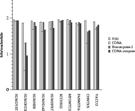
To make comparisons among entropy estimation methods clearer, figure 2 summarizes the results from table 2 for CDNA, $H_6$, BIOCOMPRESS-2, and CDNA-compress. In all cases CDNA outperforms conventional entropy estimates, and in almost all cases by a substantial margin. In many cases the compressive estimates from CDNA (i.e., CDNA-compress) are lower than those of BIOCOMPRESS-2. In several they are comparable, and in only one case (VACCG) does BIOCOMPRESS-2 outperform CDNA-compress by as much as 0.05 bits. It is possible that even this case is due to the offline nature of the current CDNA program which as mentioned above forces us to compute compressive estimates by dividing the sequence into large segments. Finally, we remark that while the table contains results for HUMRETBLAS, this sequence was used in our parameter sensitivity study below.

The CDNA program's behavior is parameterized by several values:

• The number of EM iterations to perform when learning the model's parameters based on the training set.

• The set of allowed window sizes (trailing contexts).

• The size of the training sample.

• The size of the test sample.

• The number of cross-validation segments.

• The random seed that controls all sampling.

• The distance measure to use.

The distance measure is discussed later in section 6 and for all other experiments is fixed as described earlier. We used 3-way cross-validation to assess parameter sensitivity (see discussion below), and 8-way cross-validation for all experiments. Our test samples were of size $1000$ per cross-validation segment for a total of $8000$ positions. To assess the variation due to all sampling, we performed $11$ different cross-validation estimates using different random seeds. The mean entropy estimate for HUMRETBLAS was $1.6939$ bits with a standard deviation of $0.014$ bits. Larger samples would result in smaller variance at the expense of computer time.

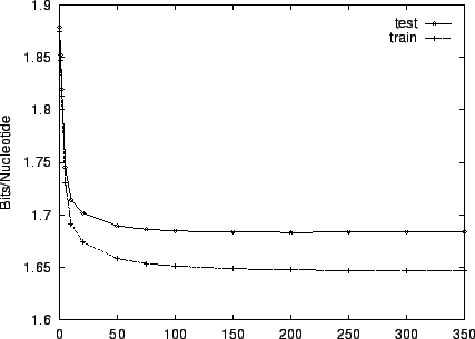
Figure 3 shows the effect of EM iterations on the entropy estimate for both training and test sets. This figure and the two that follow employ HUMRETBLAS. Based on this analysis, we chose $200$ EM iterations for our experiments. Notice that there is little overtraining. Both train and test performance are essentially constant after $150$ iterations, and their gap is small.

Figure 3: The effect of varying the number of EM learning iterations on performance for HUMRETBLAS.

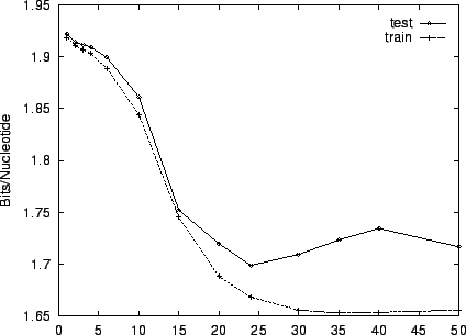
Figure 4 shows the effect of a single window size on performance. Beyond $25$, overtraining is evident. This is to be expected since the number of parameters grows quadratically with window size. For our experiments we selected a mixture of windows of size $2,4,6,8,\ldots,24$. Odd values were excluded only to reduce memory requirements for the model. Additional experiments indicated that while mixtures of different window sizes did in general help, the benefit was somewhat small. We did not study this for all sequences and therefore employed a mixture to ensure that the model is as general as possible (in theory the mixture can only help).

Figure 4: The effect of varying the trailing context size (window) on performance for HUMRETBLAS.

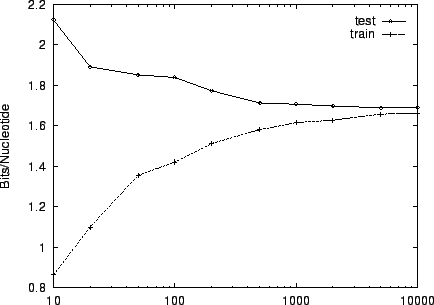
Finally, figure 5 shows the sensitivity of performance on training set size. We used a training set of size $5000$ for our experiments because beyond that point, little improvement was evident: train and test performance had essentially converged.

Figure 5: The effect of varying the size of the training set on performance for HUMRETBLAS.

Our results so far have consisted of entropy estimates for sequences of a single type. We now present the results of several cross-entropy experiments. By this we mean that the type of the training set is different from that of the test set. In table 3 mammalian coding regions and non-coding regions form the two types. A substantial cross-entropic gap is apparent. That is, a model trained on the coding sequence might be used to distinguish coding from non-coding based on entropy. The same is true when one trains on the non-coding sequence.

The same experiment produces very different results for yeast as shown in table 4. While a large gap exists when one trains using the non-coding regions, a reverse gap exists in the other case. That is, training on the coding regions assigns shorter codes to the non-coding regions, than to itself. While this effect is weak, it suggests that sequences from the coding region may be echoed in the non-coding region.

Cross-species entropy estimates are interesting in general, but our one example shown in table 5 shows little interesting structure. That is, yeast coding regions teach nothing about human coding regions and visa versa. In fact, the entropy estimates are in both cases worse than random. In the non-coding case, a weak relationship exists, but is easily explained by agreement on the low order multigraphic statistics of the sequences, e.g. $H_4$.

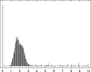
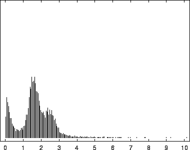
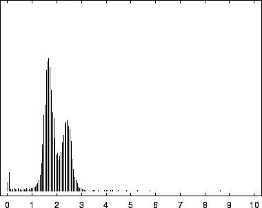
The entropy estimates we have discussed reduce to a single number the model's performance on a sequence. It represents the average code-length but says nothing about their distribution. The histograms of figures 6,7, and 8, depict this distribution for the EBV virus, the human gene HUMRETBLAS, and the yeast chromosome SCCHRIII. They present an interesting visual signature of a sequence. Trimodality is apparent in all three, but is present to a varying extent.

The first mode, most prevalent in our viral example, corresponds to near-zero code-lengths that correspond to long exact or near-exact repeats. In the viral case, this peak is particularly narrow because while the sequence is known to contain several long exact repeats, it lacks the full range of near repeats of various lengths found in sequences such as HUMRETBLAS. The middle mode corresponds to nucleotides having a long context that matches well with some other segments from the sequence. In this case short codes are assigned so long as these matches predict well the following nucleotide. The rightmost mode, particularly pronounced in SCCHRIII and less so in HUMRETBLAS, correspond to codes well over $2$ bits. Here the model had a strong prediction, but was wrong.

Figure 6: Histogram of nucleotide code-lengths for EBV.

Figure 7: Histogram of nucleotide code-lengths for HUMRETBLAS.

Figure 8: Histogram of nucleotide code-lengths for SCCHRIII (yeast).

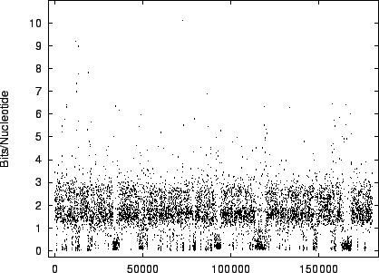
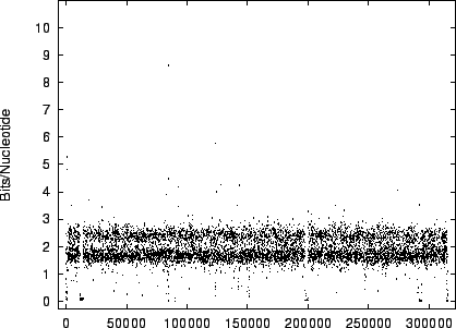
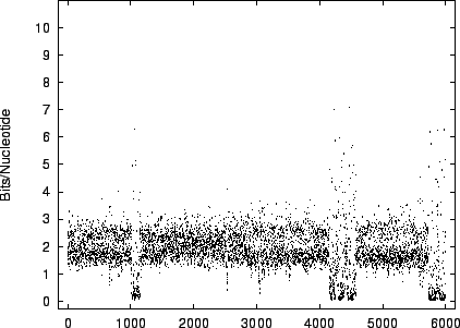
The distribution of code-lengths displayed in these histograms says nothing about how code-lengths are distributed with respect to position in the DNA sequence. To visualize this we have plotted in figures 9 and 10 the code-lengths at $8000$ random positions for HUMRETBLAS and SCCHRIII. It is apparent that the distribution is not homogeneous and presents another interesting visual signature of the sequence. The distribution for HUMRETBLAS is shown at a a closer scale (figure 11) where finer structure is revealed. The modality noted in the histograms is also apparent in these plots.

Figure 9: The variation of code-length with position for HUMRETBLAS.

Figure 10: The variation of code-length with position for SCCHRIII (yeast).

Figure 11: The variation of code-length with position for HUMRETBLAS in the first 6,000 positions.

Alternative Metrics

Our model exploits near matches to form a prediction, and its performance therefore depends on precisely what is meant by near, i.e., the distance metric used to judge string similarity. In this section we begin by discussing four metrics and report on their performance.

The simplest notion of string distance relevant to our domain is simple Hamming distance: the number of mismatching nucleotides in two strings of equal length. We will refer to this as the nucleotide-sense metric. As mentioned earlier, our domain knowledge suggests that we also compare the strings after reversing one, and complementing its bases. Both distances are computed and the smaller one used. This is our nucleotide-both metric, and was used in all experiments from earlier sections.

Coding regions have additional structure which we capture in another pair of metrics: amino-sense and amino-both. A common misconception is that coding regions should compress well because three nucleotides together ($64$ possibilities) code for only one of $21$ amino acids. This reasoning is flawed because $61$ of the $64$ possibilities represent valid codes for amino acids. Only $3$ codes are used to stop transcription. Thus the maximum entropy level for coding regions, is not $\log_2 21 \approx 1.46$ bits, nor $2$ bits as for random unconstrained sequences, but rather is $\log_2 61 / 3 \approx 1.977$ bits. In fact, it has been observed by several authors that coding regions are less compressible than non-coding regions (e.g., [Mantegna et al., 1993,Salamon and Konopka, 1992,Farach et al., 1995]). So it is clear that two sequences that code for the same polypeptide may nevertheless have large Hamming distance. The amino-sense distance between two strings whose length is a multiple of 3, and that are assumed to be aligned with the reading frame, is straightforward: it is simply the number of mismatches in the amino acid sequence coded by the nucleotide sequence; where the stop signal is considered to be a 21st amino acid.

We extend this definition to the case in which the strings being compared are not necessarily a multiple of 3 in length, and we drop the assumption that they are aligned with the reading frame. The comparison does however assume that the strings are similarly aligned. If the first string begins one base into the reading frame, it is assumed that the other string does as well. That is, the strings must be in phase. This assumption is appropriate because our search for near matches will consider all possible positions, and in so doing all relative phases.

Selected experiments comparing these four metrics are shown in table 6⁶. Entire sequences as well as their noncoding and coding regions were considered. The nucleotide-both metric performs best, and was therefore used for the experiments reported in earlier sections.

The amino metrics never outperformed their nucleotide counterparts. This is not so surprising for entire sequences, or noncoding regions, but we expected the amino metrics might perform better for coding regions. In fact their estimates are somewhat worse. Their poor performance is explained by the fact that they distinguish fewer discrete distances, and are always blind to the exact nucleotide structure of the sequence, even in the positions immediately before the base to be predicted.

The motivation in designing these metrics was the possibility that coding regions might contain long nearly identical amino acid sequences, which despite their nearness when expressed as an amino acid sequence, are far apart when coded as nucleotides. As explained above, our first attempt to capture this domain knowledge in the model was unsuccessful, so we tried another approach that produced a slightly stronger model for coding regions.

Our second approach separates the prediction problem into two stages. An amino acid is first predicted using CDNA based on inexact matches, where the sequence is viewed at the amino acid level, i.e., has alphabet size $20$. Unlike our earlier models, which make no assumption as to the nature of the DNA, this model assumes that its input is a sequence of legal codons. The model's second stage predicts a particular codon, conditioned on the already predicted amino acid, and on earlier positions which are now viewed at the nucleotide level. The codon entropy estimate is then the sum of the entropies of these two stages, and we write:

$$H(C) = H(A) + H(C\vert A)$$ (10)

Dividing $H(C)$ by three then gives a per-nucleotide entropy which may be compared with earlier results. Table 7 gives the results of several models on our non-redundant data set.

The first line of table 7 provides for reference, the entropy corresponding to a uniformly random sequence of codons. The next line reports the standard multigraphic entropy $H_6$ where alphabet is nucleotides ($H_6$ was optimal). Line three reports the result of the CDNA program operating on a sequence of nucleotides⁷. Its performance is a mere $0.01$ bits better than $H_6$. The fourth line reports the results from a two-stage model where the first stage predicts an amino acid using a simple 2-gram model (i.e., frequencies of amino acid pairs). The second stage predicts a codon, based on the predicted amino acid, and the two preceding nucleotides. In line 5, the 2-gram model is replaced with CDNA program where the alphabet is now amino acids, and windows from $1$ to $12$ amino acids are used. As for earlier experiments, the result on line five arises from 8-way cross validation. Therefore, nearby matches will not frequently contribute to a prediction. Line six employs what amounts to maximal cross validation, where a sequence element is predicted using everything else in the sequence. The same technique was used to produce figures 9-11.

It is apparent that our non-redundant collection of coding material is harder to model than the entire genes considered in earlier sections. Nevertheless we are able to improve the $1.92$ multigraphic estimate somewhat to $1.84$. It is important to note our non-redundant data set is not a random sample, but rather is closer to the worst case. We expect that lower entropy estimates would result from random samples of similar size, and remark that this was the case when we considered Mammals/Coding-only in table 2. There we reported an estimate of $1.80$ bits using CDNA at the nucleotide level.

It is possible that the addition of more domain knowledge will produce lower entropy estimates for coding regions. However, we believe that the actual entropy may be not so far below our current estimates. This is consistent with the view that the coding regions of DNA commonly amount to a highly random string, with only isolated critical regions. If much of large proteins amounts to scaffolding, and the bulk of proteins in a genome are large, then we would expect large entropies. By scaffolding we mean weakly constrained structure necessary only to ensure that the protein folds correctly, and that particular active regions are positioned properly in the resulting molecule. There are certainly many genes that code for somewhat small proteins, but since entropy is a per-base expected value, the genes that code for large proteins have proportionaly greater affect on our estimate. 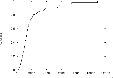Figure 12 shows that in our non-redundant collection of human genes, fewer than one third of bases are contained in coding regions of length $1000$ or less.

We conclude with a crude analysis to quantify our belief. If only the hydrophobic/hydrophilic nature of an amino acid were critical, then at most one bit would be required to make an acceptable selection. This is then $1/3$ bit per base. If, except for this structure, the string is random, then the lowest entropy we would expect is: $1.644 = 1.977 - 0.333$ bits per base. Biological experiments to quantify the sensitivity of proteins of various length to mutation, would then shed light on the actual entropy of coding regions.

Figure 12: The cumulative distribution of bases within the non-redundant human gene set, as a function of the coding region length in which they appear

Conclusion and Discussion

We have shown that the near repeats in natural DNA sequences may be incorporated into a statistical model resulting in significantly lower entropy estimates. For some sequences our model is the first to detect substantial deviations from random behavior and illustrates the importance of inexact string matching techniques in this field. It is entirely possible that very different results will be obtained, particularly for coding regions, when much more DNA is available for analysis.

It should be noted that $H_1$ entropy estimates include the known effect of $\%(C+G)$ [Gatlin, 1972] on entropy estimation, and BIOCOMPRESS-2 includes the also known effect of long exact repeats and exact complement repeats [Herzel et al., 1994]. CDNA's generally superior performance indicates that DNA possesses more structure which may be exploited.

Several notions of distance were evaluated and the best performance resulted from considering both Hamming distance to reversed and complemented targets, as well as standard Hamming distance, then selecting the minimum. We also described two-stage models crafted especially for coding regions, which perform better than our basic model on coding sequences.

Because of the observations in Section 2, a data compressor may be used as a classifier, and the result interpreted in probabilistic terms. We mention this because classification is one of the applications motivating our work. To illustrate, suppose one has two long sequences $x,y$ of DNA, the first of some type $A$ and the other of type $B$. The task is to classify a third strand $z$. Let $L(s)$ denote the bits output by the compressor when fed sequence $s$, and $s:t$ denote string concatenation. Then $L(x:z)-L(x)$ may by our remarks above be interpreted as $-\log_2 \Pr(z\vert x)$. Similarly $L(y:z)-L(y)$ corresponds to $-\log_2 \Pr(z\vert y)$. At this point one might simply compare to affect classification, or exponentiate yielding probabilities. These can then be combined along with prior class probabilities, resulting in Bayesian classifier built from data compressors.

Future work will consider stronger models exploiting additional effects. The current assumption that each prediction event is independent of the last may be dropped and a temporal dependence component added to the model. Next the metric may be enhanced to notice not only the number of mismatches, but also where they occur. Other structural changes are possible and the inclusion of additional domain knowledge in some form is a particularly interesting direction. Also, there are entirely different approaches one might take to the problem of combining experts.

Because of our interest in alternative metrics, simple linear search is used to find near matches. Our results indicate that standard Hamming distance performs well, so we plan to implement more advanced sublinear algorithms for this purpose.

Finally, we plan to investigate the application of these new, stronger models to various applications in the microbiological field.

Acknowledgments

We thank Martin Farach, Haym Hirsh, Harold Stone, and Sarah Zelikovitz for helpful comments on earlier drafts of this paper. We also thank Michiel Noordewier for the use of the large, non-redundant human gene set.

Bibliography

Baum, 1972

Baum, L. E. (1972).
An inequality and associated maximization technique in statistical estimatation of probabilistic functions of Markov processes.
Inequalities, 3:1-8.

Baum and Eagon, 1967

Baum, L. E. and Eagon, J. E. (1967).
An inequality with application to statistical estimation for probabalistic functions of a Markov process and to models for ecology.
Bull. AMS, 73:360-363.

Baum et al., 1970

Baum, L. E., Petrie, T., Soules, G., and Weiss, N. (1970).
A maximization technique occurring in the statistical analysis of probabilistic functions of Markov chains.
Ann. Math Stat., 41:164-171.

Bell et al., 1990

Bell, T. C., Cleary, J. G., and Witten, I. H. (1990).
Text Compression.
Prentice Hall.

Cardon and Stormo, 1992

Cardon, L. and Stormo, G. (1992).
Expectation maximization algorithm for identifying protein-binding sites with variable lengths from unaligned DNA fragments.
JMB, 223:159-170.

Cosmi et al., 1990

Cosmi, C., Cuomo, V., Ragosta, M., and Macchiato, M. (1990).
Characterization of nucleotidic sequences using maximum entropy techniques.
J. Theor. Biol, (147):423-432.

Cover and Thomas, 1991

Cover, T. M. and Thomas, J. A. (1991).
Elements of Information Theory.
Wiley.

Dempster et al., 1977

Dempster, A. P., Laird, N. M., and Rubin, D. B. (1977).
Maximum-likelihood from incomplete data via the EM algorithm.
J. Royal Statistical Society Ser. B (methodological), 39:1-38.

Dujon et al., 1994

Dujon, B., Alexandraki, D., Andre, B., Ansorge, W., and et al., V. B. (1994).
Complete DNA sequence of yeast chromosome XI.
Nature, 369:371-378.

Farach et al., 1995

Farach, M., Noordewier, M., Savari, S., Shepp, L., Wyner, A., and Ziv, J. (1995).
On the entropy of DNA: Algorithms and measurements based on memory and rapid convergence.
In Proceedings of the Sixth Annual ACM-SIAM Symposium on Discrete Algorithms, pages 48-57, San Francisco. SIAM/ACM-SIGACT.

Gatlin, 1972

Gatlin, L. L. (1972).
Information Theory and the Living System.
Columbia University Press, New York.

Grumbach and Tahi, 1994

Grumbach, S. and Tahi, F. (1994).
A new challenge for compression algorithms: genetic sequences.
Information Processing & Management, 30(6):875-886.

Herzel, 1988

Herzel, H. (1988).
Complexity of symbol sequences.
Syst. Anal. Modl. Simul., 5(5):435-444.

Herzel et al., 1994

Herzel, H., Ebeling, W., and Schmitt, A. (1994).
Entropies of biosequences: The role of repeats.
Physical Review E, 50(6):5061-5071.

Krogh et al., 1994

Krogh, A., Mian, I., and Haussler, D. (1994).
A hidden Markov model that finds genes in Escheria Coli DNA.
Nucleic Acids Research supplement, 22:4768-4778.

Lauc et al., 1992

Lauc, G., Ilic, I., and Heffer-Lauc, H. (1992).
Entropies of coding and noncoding sequences of DNA and proteins.
Biophysical Chemistry, (42):7-11.

Mantegna et al., 1993

Mantegna, R., Buldyrev, S., Goldberger, A., Havlin, S., Peng, C.-K., Simons, M., and Stanley, H. (1993).
Linguistic features of noncoding DNA sequences.
Physical Review Letters, 73(23):3169-3172.

Noordewier, 1996

Noordewier, M. (1996).
Private Communication. Available at http://paul.rutgers.edu/~loewenst/cdna.html.

Poritz, 1988

Poritz, A. B. (1988).
Hidden Markov models: a guided tour.
In Proc. ICASSP-88, volume 1, pages 7-13, New York. IEEE.

Redner and Walker, 1984

Redner, R. A. and Walker, H. F. (1984).
Mixture densities, maximum likelihood, and the EM algorithm.
SIAM Review, 26:195-239.

Salamon and Konopka, 1992

Salamon, P. and Konopka, A. K. (1992).
A maximum entropy principle for the distribution of local complexity in naturally occurring nucleotide sequences.
Computers Chem., 16(2):117-124.

Yianilos, 1997

Yianilos, P. N. (1997).
Topics in Computational Hidden State Modeling.
PhD thesis, Dept. of Computer Science, Princeton University.

Ziv and Lempel, 1977

Ziv, J. and Lempel, A. (1977).
A universal algorithm for sequential data compression.
IEEE Transactions on Information Theory, IT-23(3).

Table: Predicted vs. observed matches (HUMRETBLAS, window size 20). Contexts of length 20 from the first $\frac{1}{8}$ were matched to contexts in the subsequent $\frac{7}{8}$ of the gene.

Hamming	Expected		Observed		.	% hit at		.	% correct
Distance	# Matches		# Matches		.	least once		.	given 1+ hits
0	1	.	44 $\times 10^{-7}$	0	.	387	4	.	4%	90.91%
1	8	.	61 $\times 10^{-6}$	0	.	143	7	.	2	83.77
2	2	.	45 $\times 10^{-4}$	0	.	278	11	.	0	78.19
3	4	.	42 $\times 10^{-3}$	0	.	505	17	.	6	66.00
4	0	.	0563	1	.	184	33	.	2	45.91
5	0	.	541	4	.	148	78	.	2	35.86
6	4	.	01	18	.	759	98	.	3	31.90
7	24	.	3	80	.	69	100	.		29.19
8	119	.		304	.	9	100	.		28.35
9	475	.		986	.	0	100	.		28.09
10	1566	.		2713	.		100	.		27.86
11	4271	.		6286	.		100	.		27.68
12	9609	.		12300	.		100	.		27.53
13	17740	.		20172	.		100	.		27.33
14	26610	.		27387	.		100	.		27.09
15	31932	.		30356	.		100	.		26.86
16	29936	.		26813	.		100	.		26.57
17	21131	.		18200	.		100	.		26.28
18	10566	.		8931	.		100	.		25.94
19	3337	.		2826	.		100	.		25.69
20	500	.		434	.	5	100	.		25.43

Table 2: Summary of entropy estimates (bits/nucleotide).

		Algorithm
		UNIX					bio-com-	CDNA
sequence	length	compress	$H_1$	$H_4$	$H_6$	CDNA	press-2	compress
Mammals
14 Sequences	1029151	2.19	1.98	1.91	1.91	1.67
Coding only	46457	2.19	1.99	1.94	1.94	1.80
Noncoding only	982694	2.11	1.98	1.92	1.90	1.74
HUMDYSTROP	38770	2.23	1.95	1.91	1.95	1.91	1.93	1.93
HUMGHCSA	66495	2.19	2.00	1.92	1.86	0.54	1.31	0.95
HUMHBB	73308	2.20	1.97	1.91	1.92	1.68	1.88	1.77
HUMHDABCD	58864	2.21	2.00	1.92	1.89	1.63	1.88	1.67
HUMHPRTB	56737	2.20	1.97	1.91	1.90	1.69	1.91	1.72
HUMRETBLAS	180388	2.14	1.95	1.90	1.90	1.66		1.75
Yeast Chromosome III	315338	2.18	1.96	1.94	1.95	1.90	1.92	1.94
Coding only	211551	2.20	1.97	1.95	1.96	1.92
Noncoding only	103787	2.19	1.93	1.91	1.92	1.85
Mitochondria
MPOMTCG	186609	2.20	1.98	1.96	1.96	1.83	1.94	1.87
PANMTPACGA	100314	2.12	1.88	1.86	1.86	1.81	1.88	1.85
Other Eukaryotes
CEC07A9	66004	2.20	1.94	1.90	1.92	1.89
CHNTXX	155844	2.19	1.96	1.93	1.93	1.30	1.62	1.65
Prokaryotes
7 sequences	784658	2.22	2.00	1.95	1.95	1.92
Eukaryotic Viruses
5 sequences	650477	2.15	1.94	1.91	1.91	1.66
EBV	172281	2.17	1.97	1.93	1.91	1.54
VACCG	191737	2.14	1.92	1.90	1.90	1.69	1.76	1.81
Bacteriophages
3 sequences	140739	2.25	1.98	1.94	1.94	1.93

Table 3: Mammalian corpus cross-entropies (bits/nucleotide).

Training	Test Data
Set	Coding	Noncoding
Coding	1.829	2.010
Noncoding	1.949	1.727

Table 4: Yeast chromosome III cross-entropies (bits/nucleotide).

Training	Test Data
Set	Coding	Noncoding
Coding	1.941	1.918
Noncoding	1.982	1.831

Table 5: Yeast/Mammalian cross-entropies (bits/nucleotide).

Training Set	Test Set	Entropy
Mammalian Coding	Yeast Coding	2.026
Mammalian Noncoding	Yeast Noncoding	1.927
Yeast Coding	Mammalian Coding	2.033
Yeast Noncoding	Mammalian Noncoding	1.955

Table 6: Effect of metric on entropy estimate (bits/nucleotide).

	nucleotide		amino acid
sequence	sense	both	sense	both
Mammals
Coding only	1.830	1.830	1.882	1.895
Noncoding only	1.750	1.727	1.795	1.769
HUMGHCSA	0.525	0.510	0.550	0.547
HUMRETBLAS	1.748	1.686	1.799	1.731
SCCHRIII	1.904	1.879	1.930	1.926
Coding only	1.947	1.941	1.966	1.970
Noncoding only	1.879	1.831	1.889	1.850
Prokaryotes
7 sequences	1.944	1.939	1.977	1.977

Table: Summary of modeling results (bits/nucleotide) for coding regions extracted from a non-redundant collection of 490 human genes .

	Model Description	bits
1.	Max. Entropy	1.98
2.	Nucleotide 6-grams	1.92
3.	CDNA nucleotide	1.91
4.	Amino 2-grams + Codon-predict	1.89
5.	CDNA amino (8 way) + Codon-predict	1.87
6.	CDNA amino (max. way) + Codon-predict	1.84

About this document ...

Significantly Lower Entropy Estimates for Natural DNA Sequences

This document was generated using the LaTeX2HTML translator Version 2K.1beta (1.47)

Copyright © 1993, 1994, 1995, 1996, Nikos Drakos, Computer Based Learning Unit, University of Leeds.
Copyright © 1997, 1998, 1999, Ross Moore, Mathematics Department, Macquarie University, Sydney.

The command line arguments were:
latex2html -split 0 -image_type gif -nonext_page_in_navigation -noprevious_page_in_navigation -up_url ../main.html -up_title 'Publication homepage' -numbered_footnotes cdna.tex

The translation was initiated by Peter N. Yianilos on 2002-06-30

Footnotes

... bits.¹

This gap may be thought of as the mutual information between the nucleotide being predicted, and its past.

... character²

As implemented in the UNIX (registered trademark of X/Open Company, Ltd.) compress utility.

... well-behaved³

It is sufficient for example that the process be stationary and ergodic -- see the Shannon-McMillan-Breiman theorem.

... symbol⁴

Unfortunately this isn't exactly correct for all data compression schemes, e.g. for Lempel-Ziv coding. The heart of the problem is that these codes consider only the greedy parse of the sequence. By this we mean that if one sums over all sequences of length $L$ their inferred probability $2^{-\mbox{\tiny code-length}}$, one will not obtain unity. In most cases the sum is strictly less than unity and the inferred probabilities may be thought of as proportional to probabilities. The result is that entropy estimates are increased by a positive additive constant. In practice however, the discrepancy is modest and one may without harm think of codes as corresponding to probabilities.

... optima.⁵

We noted the entropy estimates of HUMRETBLAS using different randomly generated initial probability distributions. As the number of EM iterations increases, each distribution converges to a different (though similar) value (cf. Figure 3).

...table:metric⁶

These data were collected using smaller numbers of training and test samples than those presented in table 2.

... nucleotides⁷

Same parameters as for earlier experiments, but 2,000 training samples